
As soon as we open a position in the market, we are exposed to various types of risks, such as volatility risk and credit risk. To preserve our trading capital as much as possible, it is important to incorporate some form of risk management measures to our trading system.
Perhaps the most common measure of risk used in the financial industry is the VaR technique. It is designed to simply answer: what is the worst expected amount of loss, given a specific probability level, say 95 percent, over a certain period of time? The beauty of VaR is that it can be applied to multiple levels, from position-specific micro level to portfolio-based macro level. For example, a VaR of $1 million with a 95 percent confidence level for a one-day time horizon states that on average, only 1 day out of 20 would you expect to lose more than $1 million due to market movements.
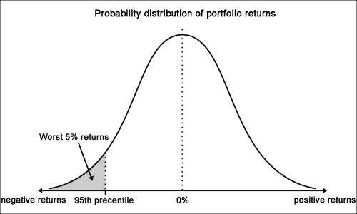
The following figure illustrates a normally distributed portfolio returns with a mean of 0 percent, where VaR is the loss corresponding to the 95th percentile of the distribution of portfolio returns:
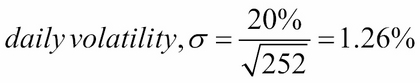
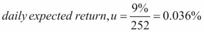
Suppose we have $100 million under management at a fund claiming to have the same risk as an S&P 500 index fund, with an expected return of 9 percent and a standard deviation of 20 percent. To calculate the daily VaR at the 5 percent risk level or 95 percent confidence using the variance-covariance method, we will use the following formulas:
Here, P is the value of the portfolio, and ![]() is the inverse normal probability distribution with risk level of
is the inverse normal probability distribution with risk level of ![]() , mean of
, mean of ![]() , and standard deviation of
, and standard deviation of ![]() . The number of trading days per year is assumed to be 252. It turns out that the VaR is $2,036,606.50.
. The number of trading days per year is assumed to be 252. It turns out that the VaR is $2,036,606.50.
However, the use of VaR is not without its flaws. It does not take into account the probability of the loss for extreme events happening on the far ends of the tails on the normal distribution curve. The magnitude of the loss beyond a certain VaR level would be difficult to estimate as well. The VaR that we investigated uses historical data and an assumed constant volatility level. Such measures are not indicative of our future performance.
Let's take a practical approach to calculate the daily VaR of a set of stock prices from Yahoo! Finance. We will investigate the AAPL stock:
import datetime as dt
import numpy as np
import pandas.io.data as rda
from scipy.stats import norm

def calculate_daily_VaR(P, prob, mean, sigma,
                        days_per_year=252.):
    min_ret = norm.ppf(1-prob,
                       mean/days_per_year,
                       sigma/np.sqrt(days_per_year))
    return P - P*(min_ret+1)

if __name__ == "__main__":
    start = dt.datetime(2013, 12, 1)
    end = dt.datetime(2014, 12, 1)

    prices = rda.DataReader("AAPL", "yahoo", start, end)
    returns = prices["Adj Close"].pct_change().dropna()

    portvolio_value = 100000000.00
    confidence = 0.95
    mu = np.mean(returns)
    sigma = np.std(returns)

    VaR = calculate_daily_VaR(portvolio_value, confidence,
                              mu, sigma)
    print "Value-at-Risk:", round(VaR, 2)
The calculate_daily_VaR function performs the daily VaR calculation, assuming 252 trading days per year. The mean and sigma variables are annualized values of the average and standard deviation of daily stock returns respectively. The norm.ppf method of the scipy.stats module performs the inverse of the normal probability with a risk level of 1-prob, where prob is the confidence value of interest.
The pandas.io.data.DataReader function is a nifty feature of pandas that provides remote data access to certain data sources, including the following:
- Yahoo! Finance
- Google Finance
- St. Louis Fed (FRED)
- Kenneth French's data library
- World Bank
- Google Analytics
We chose Yahoo! Finance with the yahoo value encapsulated in string quotes in the function arguments, along with the start and end dates of the data. The Adj Close column of the returned DataFrame object is used to compute the daily percentage price changes. Finally, we will call the calculate_daily_VaR function to compute our daily VaR:
Value-at-Risk: 138755.57
The daily VaR for the stock AAPL with 95 percent confidence is $138,755.57.