
In this section, we will take a look at pricing a callable bond. We assume that the bond to be priced is a zero-coupon paying bond with an embedded European call option. The price of a callable bond can be thought of as:
The value of a zero-coupon bond with a par value of 1 at time ![]() and prevailing interest rate
and prevailing interest rate ![]() is defined as:
is defined as:
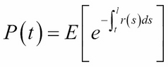
Since the interest rate ![]() is always changing, we will rewrite the zero-coupon bond as:
is always changing, we will rewrite the zero-coupon bond as:

Now, the interest rate ![]() is a stochastic process that accounts for the price of the bond from time
is a stochastic process that accounts for the price of the bond from time t to T, where T is the time to maturity of the zero-coupon bond.
To model the interest rate ![]() we can use one of the short rate models as discussed in this chapter as a stochastic process. For this purpose, we will use the Vasicek model to model the short rate process.
we can use one of the short rate models as discussed in this chapter as a stochastic process. For this purpose, we will use the Vasicek model to model the short rate process.
The expectation of a log-normally distributed variable ![]() is given by:
is given by:
Taking moments of the log-normally distributed variable X:

We obtained the expected value of a log-normally distributed variable, which we will use in the interest rate process for the zero-coupon bond.
Remember the Vasicek short-rate process model:
Then, r(t) is derived as:
Using the characteristic equation and the interest rate movements of the Vasicek model, we can rewrite the zero-coupon bond price in terms of expectations:
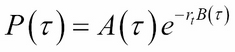
Here:
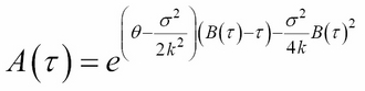
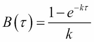
The Python implementation of the zero-coupon bond price is given in the ExactZCB function:
import numpy as np
""" Get zero coupon bond price by Vasicek model """
def exact_zcb(theta, kappa, sigma, tau, r0=0.):
B = (1 - np.exp(-kappa*tau)) / kappa
A = np.exp((theta-(sigma**2)/(2*(kappa**2))) *
(B-tau) - (sigma**2)/(4*kappa)*(B**2))
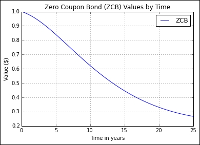
return A * np.exp(-r0*B)For example, we are interested in finding out the prices of zero-coupon bond prices for a number of maturities. We model the Vasicek short-rate process with a theta value of 0.5, kappa value of 0.02, sigma value of 0.02, and an initial interest rate r0 of 0.015. Plugging these values into the ExactZCB function, we obtain zero-coupon bond prices, for the time period from 0 to 25 years with intervals of 0.5 years, and plot out the graph:
>>> Ts = np.r_[0.0:25.5:0.5]
>>> zcbs = [exact_zcb(0.5, 0.02, 0.03, t, 0.015) for t in Ts]
>>>
>>> import matplotlib.pyplot as plt
>>> plt.title("Zero Coupon Bond (ZCB) Values by Time")
>>> plt.plot(Ts, zcbs, label='ZCB')
>>> plt.ylabel("Value ($)")
>>> plt.xlabel("Time in years")
>>> plt.legend()
>>> plt.grid(True)
>>> plt.show()
The following graph is the output for the preceding commands:
Issuers of callable bonds may redeem the bond at an agreed price as specified in the contract. To price such a bond, the discounted early-exercise values can be defined as:
Here, ![]() is the price ratio of the strike price to the par value and
is the price ratio of the strike price to the par value and ![]() is the interest rate for the strike price.
is the interest rate for the strike price.
The Python implementation of the early-exercise option can then be written as follows:
import math
def exercise_value(K, R, t):
    return K*math.exp(-R*t)
In the preceding example, we are interested in valuing a call option with a strike ratio of 0.95 and an initial interest rate of 1.5 percent. We can then plot the values as a function of time and superimpose them onto a graph of zero-coupon bond prices to give us a better visual representation of the relationship between zero-coupon bond prices and callable bond prices:
>>> Ts = np.r_[0.0:25.5:0.5]
>>> Ks = [exercise_value(0.95, 0.015, t) for t in Ts]

>>> zcbs = [exact_zcb(0.5, 0.02, 0.03, t, 0.015) for t in Ts]
>>> import matplotlib.pyplot as plt
>>> plt.title("Zero Coupon Bond (ZCB) "
...           "and Strike (K) Values by Time")
>>> plt.plot(Ts, zcbs, label='ZCB')
>>> plt.plot(Ts, Ks, label='K', linestyle="--", marker=".")
>>> plt.ylabel("Value ($)")
>>> plt.xlabel("Time in years")
>>> plt.legend()
>>> plt.grid(True)
>>> plt.show()
Here is the output for the preceding commands:
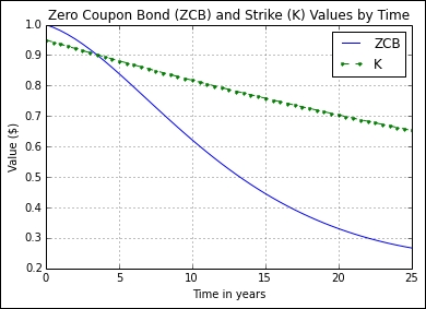
From the preceding graph, we can approximate the price of callable zero-coupon bond prices. Since the bond issuer owns the call, the price of the callable zero-coupon bond can be stated as:
This callable bond price is an approximation, given the current interest rate level. The next step would be to treat early-exercise by going through a form of policy iteration, which is a cycle used to determine optimum early-exercise values and their effect on other nodes, and check whether they become due for an early exercise. In practice, such an iteration only occurs once.
So far, we have used the Vasicek model in our short rate process for modeling a zero-coupon bond. We can undergo policy iteration by finite differences to check for early-exercise conditions and their effect on other nodes. We will use the implicit method of finite differences for the numerical pricing procedure, as discussed in Chapter 4, Numerical Procedures.
Let's create a class named VasicekCZCB that will incorporate all the methods used for implementing the pricing of callable zero-coupon bonds by the Vasicek model. The full Python code of this class can be found at the end of this section.
The methods used are as follows:
vasicek_czcb_values(self, r0, R, ratio, T, sigma, kappa, theta, M, prob=1e-6, max_policy_iter=10, grid_struct_const=0.25, rs=None): This method is the point of entry to kick-start the pricing process. The variabler0is the short-rate at time ;
; Ris the strike zero rate for the bond price;ratiois the strike price per par value of the bond;Tis the time to maturity;sigmais the volatility of the short rate ;
; kappais the rate of mean reversion;thetais the mean of the short rate process;Mis the number of steps in the finite differences scheme,probis the probability on the normal distribution curve used by thevasicek_limitsmethod to determine short rates;max_policy_iteris the maximum number of policy iterations used to find early-exercise nodes;grid_struct_constis the maximum threshold ofdtmovement that determinesNin thecalculate_Nmethod; andrsis the list of interest rates from which the short rate process follows. This method returns a list of evenly spaced short rates and a list of option prices.vasicek_params(self, r0, M, sigma, kappa, theta, T, prob, grid_struct_const=0.25, rs=None): This method computes the implicit scheme parameters for the Vasicek model. It returns comma-separated values ofr_min,dr,N, anddt. If no value is supplied tors, values ofr_mintor_maxwill be automatically generated by thevasicek_limitsmethod as a function ofprobfollowing a normal distribution.vasicek_limits(self, r0, sigma, kappa, theta, T, prob=1e-6): This method computes the minimum and maximum of the Vasicek interest rate process by a normal distribution process. The expected value of the short rate processr(t)under the Vasicek model is given as: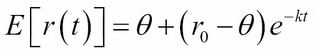
The variance is defined as:
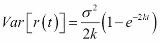
The function returns a tuple of the minimum and maximum interest rate level as defined by the probability for the normal distribution process.
vasicek_diagonals(self, sigma, kappa, theta, r_min, dr, N, dtau): This method returns the diagonals of the implicit scheme of finite differences, where: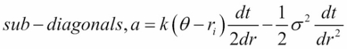
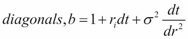
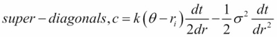
The boundary conditions are implemented using Neumann boundary conditions.
check_exercise(self, V, eex): This method returns a list of Boolean values, indicating the indices suggesting optimum payoff from an early exercise.exercise_call_price(self, R, ratio, tau): This method returns the discounted value of the strike price as a ratio.vasicek_policy_diagonals(self, subdiagonal, diagonal, superdiagonal, v_old, v_new, eex): This method is used by the policy iteration procedure that updates the sub-diagonals, diagonals, and super diagonals for one iteration. In indices, where an early exercise is carried out, the sub-diagonals and super diagonals will have these values set to 0 and the remaining values on the diagonal. The method returns comma-separated values of the new sub-diagonal, diagonal, and super-diagonal values.iterate(self, subdiagonal, diagonal, superdiagonal, v_old, eex, max_policy_iter=10): This method performs the implicit scheme of finite differences by performing a policy iteration, where each cycle involves solving the tridiagonal systems of equations, calling thevasicek_policy_diagonalsmethod to update the three diagonals, and returns the callable zero-coupon bond price if there are no further early-exercise opportunities. It also returns the number of policy iterations performed.tridiagonal_solve(self, a, b, c, d): This method is the implementation of the Thomas algorithm for solving tridiagonal systems of equations. The systems of equations may be written as:
This equation is represented in matrix form:
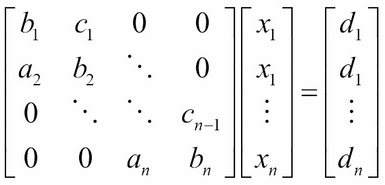
Here, a is a list for the sub-diagonals, b is a list for the diagonal, and c is the super diagonal of the matrix.
With these methods defined, we can now run our code and price a callable zero-coupon bond by the Vasicek model.
The implementation of the VasicekCZCB class in Python is given as follows:
""" Price a callable zero coupon bond by the Vasicek model """
import math
import numpy as np
import scipy.stats as st


class VasicekCZCB:

    def __init__(self):
        self.norminv = st.distributions.norm.ppf
        self.norm = st.distributions.norm.cdf

    def vasicek_czcb_values(self, r0, R, ratio, T, sigma, kappa,
                            theta, M, prob=1e-6, max_policy_iter=10,
                            grid_struct_const=0.25, rs=None):
        r_min, dr, N, dtau =
            self.vasicek_params(r0, M, sigma, kappa, theta,
                                T, prob, grid_struct_const, rs)
        r = np.r_[0:N]*dr + r_min
        v_mplus1 = np.ones(N)

        for i in range(1, M+1):
            K = self.exercise_call_price(R, ratio, i*dtau)
            eex = np.ones(N)*K
            subdiagonal, diagonal, superdiagonal =
                self.vasicek_diagonals(sigma, kappa, theta,
                                       r_min, dr, N, dtau)
            v_mplus1, iterations =
                self.iterate(subdiagonal, diagonal, superdiagonal,
                             v_mplus1, eex, max_policy_iter)
        return r, v_mplus1

    def vasicek_params(self, r0, M, sigma, kappa, theta, T,
                       prob, grid_struct_const=0.25, rs=None):
        (r_min, r_max) = (rs[0], rs[-1]) if not rs is None
            else self.vasicek_limits(r0, sigma, kappa,
                                     theta, T, prob)
        dt = T/float(M)
        N = self.calculate_N(grid_struct_const, dt,
                             sigma, r_max, r_min)
        dr = (r_max-r_min)/(N-1)
        return r_min, dr, N, dt

    def calculate_N(self, max_structure_const, dt,
                    sigma, r_max, r_min):
        N = 0
        while True:
            N += 1
            grid_structure_interval = dt*(sigma**2)/(
                ((r_max-r_min)/float(N))**2)
            if grid_structure_interval > max_structure_const:
                break

        return N

    def vasicek_limits(self, r0, sigma, kappa,
                       theta, T, prob=1e-6):
        er = theta+(r0-theta)*math.exp(-kappa*T)
        variance = (sigma**2)*T if kappa==0 else
                    (sigma**2)/(2*kappa)*(1-math.exp(-2*kappa*T))
        stdev = math.sqrt(variance)
        r_min = self.norminv(prob, er, stdev)
        r_max = self.norminv(1-prob, er, stdev)
        return r_min, r_max

    def vasicek_diagonals(self, sigma, kappa, theta,
                          r_min, dr, N, dtau):
        rn = np.r_[0:N]*dr + r_min
        subdiagonals = kappa*(theta-rn)*dtau/(2*dr) -
                       0.5*(sigma**2)*dtau/(dr**2)
        diagonals = 1 + rn*dtau + sigma**2*dtau/(dr**2)
        superdiagonals = -kappa*(theta-rn)*dtau/(2*dr) -
                         0.5*(sigma**2)*dtau/(dr**2)

        # Implement boundary conditions.
        if N > 0:
            v_subd0 = subdiagonals[0]
            superdiagonals[0] = superdiagonals[0] -
                                subdiagonals[0]
            diagonals[0] += 2*v_subd0
            subdiagonals[0] = 0

        if N > 1:
            v_superd_last = superdiagonals[-1]
            superdiagonals[-1] = superdiagonals[-1] -
                                 subdiagonals[-1]
            diagonals[-1] += 2*v_superd_last
            superdiagonals[-1] = 0

        return subdiagonals, diagonals, superdiagonals

    def check_exercise(self, V, eex):
        return V > eex

    def exercise_call_price(self, R, ratio, tau):
        K = ratio*np.exp(-R*tau)
        return K

    def vasicek_policy_diagonals(self, subdiagonal, diagonal,
                                 superdiagonal, v_old, v_new, eex):
        has_early_exercise = self.check_exercise(v_new, eex)
        subdiagonal[has_early_exercise] = 0
        superdiagonal[has_early_exercise] = 0
        policy = v_old/eex
        policy_values = policy[has_early_exercise]
        diagonal[has_early_exercise] = policy_values
        return subdiagonal, diagonal, superdiagonal

    def iterate(self, subdiagonal, diagonal, superdiagonal,
                v_old, eex, max_policy_iter=10):
        v_mplus1 = v_old
        v_m = v_old
        change = np.zeros(len(v_old))
        prev_changes = np.zeros(len(v_old))

        iterations = 0
        while iterations <= max_policy_iter:
            iterations += 1

            v_mplus1 = self.tridiagonal_solve(subdiagonal, diagonal,
                                              superdiagonal, v_old)
            subdiagonal, diagonal, superdiagonal =
                self.vasicek_policy_diagonals(subdiagonal, diagonal,
                                              superdiagonal, v_old,
                                              v_mplus1, eex)

            is_eex = self.check_exercise(v_mplus1, eex)
            change[is_eex] = 1

            if iterations > 1:
                change[v_mplus1 != v_m] = 1

            is_no_more_eex = False if True in is_eex else True
            if is_no_more_eex:
                break

            v_mplus1[is_eex] = eex[is_eex]
            changes = (change == prev_changes)

            is_no_further_changes = all((x == 1) for x in changes)
            if is_no_further_changes:
                break

            prev_changes = change
            v_m = v_mplus1

        return v_mplus1, (iterations-1)

    def tridiagonal_solve(self, a, b, c, d):
        nf = len(a)  # Number of equations
        ac, bc, cc, dc = map(np.array, (a, b, c, d))  # Copy the array
        for it in xrange(1, nf):
            mc = ac[it]/bc[it-1]
            bc[it] = bc[it] - mc*cc[it-1]
            dc[it] = dc[it] - mc*dc[it-1]

        xc = ac
        xc[-1] = dc[-1]/bc[-1]

        for il in xrange(nf-2, -1, -1):
            xc[il] = (dc[il]-cc[il]*xc[il+1])/bc[il]

        del bc, cc, dc  # Delete variables from memory

        return xc
Assume that we run this model with the parameters: r0 is 0.05, R is 0.05, ratio is 0.95, sigma is 0.03, kappa is 0.15, theta is 0.05, prob is 1e-6, M is 250, max_policy_iter is 10, grid_struc_interval is 0.25, and we are interested in the values of the interest rates between 0 percent and 2 percent. The following Python code demonstrates this model for maturities of 1 year, 5 years, 7 years, 10 years, and 20 years:
>>> r0 = 0.05
>>> R = 0.05
>>> ratio = 0.95
>>> sigma = 0.03
>>> kappa = 0.15
>>> theta = 0.05
>>> prob = 1e-6
>>> M = 250
>>> max_policy_iter=10
>>> grid_struct_interval = 0.25
>>> rs = np.r_[0.0:2.0:0.1]
>>>
>>> Vasicek = VasicekCZCB()
>>> r, vals = Vasicek.vasicek_czcb_values(r0, R, ratio, 1.,
...                                       sigma, kappa, theta,
...                                       M, prob,
...                                       max_policy_iter,
...                                       grid_struct_interval,
...                                       rs)
>>>
>>> import matplotlib.pyplot as plt
>>> plt.title("Callable Zero Coupon Bond Values by r")
>>> plt.plot(r, vals, label='1 yr')
>>>
>>> for T in [5., 7., 10., 20.]:
...
    r, vals =
...         Vasicek.vasicek_czcb_values(r0, R, ratio, T,
...                                     sigma, kappa,
                                        theta, M, prob,
...                                     max_policy_iter,
...                                     grid_struct_interval,
...                                     rs)
...     plt.plot(r, vals, label=str(T)+' yr',
...              linestyle="--", marker=".")
>>>
>>> plt.ylabel("Value ($)")
>>> plt.xlabel("r")
>>> plt.legend()
>>> plt.grid(True)
>>> plt.show()
After running the preceding commands, you get the following output:
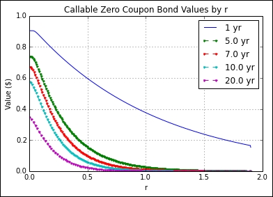
We obtained the theoretical values of pricing callable zero-coupon bonds for various maturities for various interest rates.
In pricing callable zero-coupon bonds, we used the Vasicek interest rate process to model interest rate movement with the aid of a normal distribution process. We have earlier demonstrated that the Vasicek model can produce negative interest rates, which may not be practical for most economic cycles. Quantitative analysts often use more than one model in derivative pricing to obtain realistic results as much as possible. The CIR and Hull-White models are some of the commonly discussed models in financial studies. The limitation on these models is that they involve only one factor, or a single source of uncertainty.
We also looked at the implicit scheme of finite differences for policy iteration of the early exercise. Another method of consideration is the Crank-Nicolson method of finite differences. Other methods include the Monte Carlo simulation for calibration of this model.
Finally, we obtained a final list of short rates and callable bond prices. To infer a fair value of the callable bond for a particular short rate, interpolation of the list of bond prices is required. Often, the linear interpolation method is used. Other interpolation methods of consideration are the cubic and spline interpolation methods.