
In binomial trees, each node recombines at every alternative node. In trinomial trees, each node recombines at every other node. This property of recombining trees can also be represented as lattices to help you save memory without recomputing and storing recombined nodes.
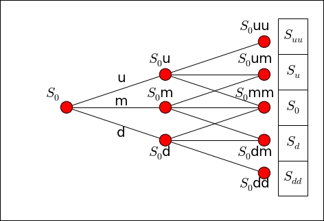
We will create a binomial lattice from the binomial CRR tree since, at every alternate up and down nodes, the prices recombine to the same probability of ![]() . In the following figure,
. In the following figure, ![]() and
and ![]() recombine with
recombine with ![]() . The tree can now be represented as a single list:
. The tree can now be represented as a single list:

For a N-step binomial, a list of size ![]() is required to contain the information on the underlying stock prices. For European option pricing, the odd nodes of payoffs from the list represent the option value upon maturity. The tree traverses backward to obtain the option value. For American option pricing, as the tree traverses backward, both ends of the list shrink, and the odd nodes represent the associated stock prices for any time step. Payoffs from the earlier exercise can then be taken into account.
is required to contain the information on the underlying stock prices. For European option pricing, the odd nodes of payoffs from the list represent the option value upon maturity. The tree traverses backward to obtain the option value. For American option pricing, as the tree traverses backward, both ends of the list shrink, and the odd nodes represent the associated stock prices for any time step. Payoffs from the earlier exercise can then be taken into account.
Let's convert the binomial tree pricing into a lattice by CRR. We can inherit from the BinomialCRROption (which in turn inherits the BinomialTreeOption class) class and create a new class named BinomialCRRLattice. The following methods are overwritten with the implementation of the lattice while retaining the behavior of all the other pricing functions:
_setup_parameters_: This method is overwritten to initialize the CRR parameters of the parent class as well as declaring the new variableMas the list size._initialize_stock_price_tree_: This method is overwritten to set up a one-dimensional NumPy array as the lattice with the sizeM._initialize_payoffs_tree_and__check_early_exercise__: These methods are overwritten to take into account the payoffs at odd nodes only.
Save this code to a file named BinomialCRRLattice.py:
""" Price an option by the binomial CRR lattice """
from BinomialCRROption import BinomialCRROption
import numpy as np


class BinomialCRRLattice(BinomialCRROption):

    def _setup_parameters_(self):
        super(BinomialCRRLattice, self)._setup_parameters_()
        self.M = 2*self.N + 1

    def _initialize_stock_price_tree_(self):
        self.STs = np.zeros(self.M)
        self.STs[0] = self.S0 * self.u**self.N

        for i in range(self.M)[1:]:
            self.STs[i] = self.STs[i-1]*self.d

    def _initialize_payoffs_tree_(self):
        odd_nodes = self.STs[::2]
        return np.maximum(
            0, (odd_nodes - self.K) if self.is_call
            else(self.K - odd_nodes))

    def __check_early_exercise__(self, payoffs, node):
        self.STs = self.STs[1:-1]  # Shorten the ends of the list
        odd_STs = self.STs[::2]
        early_ex_payoffs =
            (odd_STs-self.K) if self.is_call
            else (self.K-odd_STs)
        payoffs = np.maximum(payoffs, early_ex_payoffs)

        return payoffs
Using the same stock information from our binomial CRR model example, we can price an European and American put option using the binomial lattice pricing:
>>> from BinomialCRRLattice import BinomialCRRLattice
>>> eu_option = BinomialCRRLattice(
...     50, 50, 0.05, 0.5, 2,
...     {"sigma": 0.3, "is_call": False})
>>> print "European put: %s" % eu_option.price()
European put: 3.1051473413
>>> am_option = BinomialCRRLattice(
...     50, 50, 0.05, 0.5, 2,
...     {"sigma": 0.3, "is_call": False, "is_eu": False})
>>> print "American put: %s" % am_option.price()
American put: 3.4091814964
The trinomial lattice works in very much the same way as the binomial lattice. Since each node recombines at every other node instead of alternate nodes, extracting odd nodes from the list is not necessary. As the size of the list is the same as the one in the binomial lattice, there are no extra storage requirements in trinomial lattice pricing, as explained in the following figure:
In Python, let's create a class named TrinomialLattice for the trinomial lattice implementation that inherits from the TrinomialTreeOption class.
Just as we did for the BinomialCRRLattice class, the _setup_parameters_, _initialize_stock_price_tree_, _initialize_payoffs_tree_, and __check_early_exercise__ methods are overwritten without having to take into account the payoffs at odd nodes:
""" Price an option by the trinomial lattice """
from TrinomialTreeOption import TrinomialTreeOption
import numpy as np


class TrinomialLattice(TrinomialTreeOption):

    def _setup_parameters_(self):
        super(TrinomialLattice, self)._setup_parameters_()
        self.M = 2*self.N+1

    def _initialize_stock_price_tree_(self):
        self.STs = np.zeros(self.M)
        self.STs[0] = self.S0 * self.u**self.N

        for i in range(self.M)[1:]:
            self.STs[i] = self.STs[i-1]*self.d

    def _initialize_payoffs_tree_(self):
        return np.maximum(
            0, (self.STs-self.K) if self.is_call
            else(self.K-self.STs))

    def __check_early_exercise__(self, payoffs, node):
        self.STs = self.STs[1:-1]  # Shorten the ends of the list
        early_ex_payoffs =
            (self.STs-self.K) if self.is_call
            else(self.K-self.STs)
        payoffs = np.maximum(payoffs, early_ex_payoffs)

        return payoffs
Using the same examples as before, we can price the European and American options using the trinomial lattice model:
>>> from TrinomialLattice import TrinomialLattice
>>> eu_option = TrinomialLattice(
...     50, 50, 0.05, 0.5, 2,
...     {"sigma": 0.3, "is_call":False})
>>> print "European put: %s" % eu_option.price()
European put: 3.33090549176
>>> am_option = TrinomialLattice(
...     50, 50, 0.05, 0.5, 2,
>>> {"sigma": 0.3, "is_call": False, "is_eu": False})
>>> print "American put: %s" % am_option.price()
American put: 3.48241453902
The output agrees with the results obtained from the trinomial tree option pricing model.