22
Deep Reinforcement Learning – Building a Trading Agent
In this chapter, we'll introduce reinforcement learning (RL), which takes a different approach to machine learning (ML) than the supervised and unsupervised algorithms we have covered so far. RL has attracted enormous attention as it has been the main driver behind some of the most exciting AI breakthroughs, like AlphaGo. David Silver, AlphaGo's creator and the lead RL researcher at Google-owned DeepMind, recently won the prestigious 2019 ACM Prize in Computing "for breakthrough advances in computer game-playing." We will see that the interactive and online nature of RL makes it particularly well-suited to the trading and investment domain.
RL models goal-directed learning by an agent that interacts with a typically stochastic environment that the agent has incomplete information about. RL aims to automate how the agent makes decisions to achieve a long-term objective by learning the value of states and actions from a reward signal. The ultimate goal is to derive a policy that encodes behavioral rules and maps states to actions.
RL is considered most similar to human learning that results from taking actions in the real world and observing the consequences. It differs from supervised learning because it optimizes the agent's behavior one trial-and-error experience at a time based on a scalar reward signal, rather than by generalizing from correctly labeled, representative samples of the target concept. Moreover, RL does not stop at making predictions. Instead, it takes an end-to-end perspective on goal-oriented decision-making by including actions and their consequences.
In this chapter, you will learn how to formulate an RL problem and apply various solution methods. We will cover model-based and model-free methods, introduce the OpenAI Gym environment, and combine deep learning with RL to train an agent that navigates a complex environment. Finally, we'll show you how to adapt RL to algorithmic trading by modeling an agent that interacts with the financial market to optimize its profit objective.
More specifically, after reading this chapter, you will be able to:
- Define a Markov decision problem (MDP)
- Use value and policy iteration to solve an MDP
- Apply Q-learning in an environment with discrete states and actions
- Build and train a deep Q-learning agent in a continuous environment
- Use OpenAI Gym to train an RL trading agent
You can find the code samples for this chapter and links to additional resources in the corresponding directory of the GitHub repository. The notebooks include color versions of the images.
Elements of a reinforcement learning system
RL problems feature several elements that set them apart from the ML settings we have covered so far. The following two sections outline the key features required for defining and solving an RL problem by learning a policy that automates decisions. We'll use the notation and generally follow Reinforcement Learning: An Introduction (Sutton and Barto 2018) and David Silver's UCL Courses on RL (https://www.davidsilver.uk/teaching/), which are recommended for further study beyond the brief summary that the scope of this chapter permits.
RL problems aim to solve for actions that optimize the agent's objective, given some observations about the environment. The environment presents information about its state to the agent, assigns rewards for actions, and transitions the agent to new states, subject to probability distributions the agent may or may not know. It may be fully or partially observable, and it may also contain other agents. The structure of the environment has a strong impact on the agent's ability to learn a given task, and typically requires significant up-front design effort to facilitate the training process.
RL problems differ based on the complexity of the environment's state and agent's action spaces, which can be either discrete or continuous. Continuous actions and states, unless discretized, require machine learning to approximate a functional relationship between states, actions, and their values. They also require generalization because the agent almost certainly experiences only a subset of the potentially infinite number of states and actions during training.
Solving complex decision problems usually requires a simplified model that isolates the key aspects. Figure 22.1 highlights the salient features of an RL problem. These typically include:
- Observations by the agent on the state of the environment
- A set of actions available to the agent
- A policy that governs the agent's decisions

Figure 22.1: Components of an RL system
In addition, the environment emits a reward signal (that may be negative) as the agent's action leads to a transition to a new state. At its core, the agent usually learns a value function that informs its judgment of the available actions. The agent's objective function processes the reward signal and translates the value judgments into an optimal policy.
The policy – translating states into actions
At any point in time, the policy defines the agent's behavior. It maps any state the agent may encounter to one or several actions. In an environment with a limited number of states and actions, the policy can be a simple lookup table that's filled in during training.
With continuous states and actions, the policy takes the form of a function that machine learning can help to approximate. The policy may also involve significant computation, as in the case of AlphaZero, which uses tree search to decide on the best action for a given game state. The policy may also be stochastic and assign probabilities to actions, given a state.
Rewards – learning from actions
The reward signal is a single value that the environment sends to the agent at each time step. The agent's objective is typically to maximize the total reward received over time. Rewards can also be a stochastic function of the state and the actions. They are typically discounted to facilitate convergence and reflect the time decay of value.
Rewards are the only way for the agent to learn about the value of its decisions in a given state and to modify the policy accordingly. Due to its critical impact on the agent's learning, the reward signal is often the most challenging part of designing an RL system.
Rewards need to clearly communicate what the agent should accomplish (as opposed to how it should do so) and may require domain knowledge to properly encode this information. For example, the development of a trading agent may need to define rewards for buy, hold, and sell decisions. These may be limited to profit and loss, but also may need to include volatility and risk considerations, such as drawdown.
The value function – optimal choice for the long run
The reward provides immediate feedback on actions. However, solving an RL problem requires decisions that create value in the long run. This is where the value function comes in: it summarizes the utility of states or of actions in a given state in terms of their long-term reward.
In other words, the value of a state is the total reward an agent can expect to obtain in the future when starting in that state. The immediate reward may be a good proxy of future rewards, but the agent also needs to account for cases where low rewards are followed by much better outcomes that are likely to follow (or the reverse).
Hence, value estimates aim to predict future rewards. Rewards are the key inputs, and the goal of making value estimates is to achieve more rewards. However, RL methods focus on learning accurate values that enable good decisions while efficiently leveraging the (often limited) experience.
There are also RL approaches that do not rely on value functions, such as randomized optimization methods like genetic algorithms or simulated annealing, which aim to find optimal behaviors by efficiently exploring the policy space. The current interest in RL, however, is mostly driven by methods that directly or indirectly estimate the value of states and actions.
Policy gradient methods are a new development that relies on a parameterized, differentiable policy that can be directly optimized with respect to the objective using gradient descent (Sutton et al. 2000). See the resources on GitHub that include abstracts of key papers and algorithms beyond the scope of this chapter.
With or without a model – look before you leap?
Model-based RL approaches learn a model of the environment to allow the agent to plan ahead by predicting the consequences of its actions. Such a model may be used, for example, to predict the next state and reward based on the current state and action. This is the basis for planning, that is, deciding on the best course of action by considering possible futures before they materialize.
Simpler model-free methods, in contrast, learn from trial and error. Modern RL methods span the gamut from low-level trial-and-error methods to high-level, deliberative planning. The right approach depends on the complexity and learnability of the environment.
How to solve reinforcement learning problems
RL methods aim to learn from experience how to take actions that achieve a long-term goal. To this end, the agent and the environment interact over a sequence of discrete time steps via the interface of actions, state observations, and rewards described in the previous section.
Key challenges in solving RL problems
Solving RL problems requires addressing two unique challenges: the credit-assignment problem and the exploration-exploitation trade-off.
Credit assignment
In RL, reward signals can occur significantly later than actions that contributed to the result, complicating the association of actions with their consequences. For example, when an agent takes 100 different positions and trades repeatedly, how does it realize that certain holdings performed much better than others if it only learns about the portfolio return?
The credit-assignment problem is the challenge of accurately estimating the benefits and costs of actions in a given state, despite these delays. RL algorithms need to find a way to distribute the credit for positive and negative outcomes among the many decisions that may have been involved in producing it.
Exploration versus exploitation
The dynamic and interactive nature of RL implies that the agent needs to estimate the value of the states and actions before it has experienced all relevant trajectories. While it is able to select an action at any stage, these decisions are based on incomplete learning, yet generate the agent's first insights into the optimal choices of its behavior.
Partial visibility into the value of actions creates the risk of decisions that only exploit past (successful) experience rather than exploring uncharted territory. Such choices limit the agent's exposure and prevent it from learning an optimal policy.
An RL algorithm needs to balance this exploration-exploitation trade-off—too little exploration will likely produce biased value estimates and suboptimal policies, whereas too little exploitation prevents learning from taking place in the first place.
Fundamental approaches to solving RL problems
There are numerous approaches to solving RL problems, all of which involve finding rules for the agent's optimal behavior:
- Dynamic programming (DP) methods make the often unrealistic assumption of complete knowledge of the environment, but they are the conceptual foundation for most other approaches.
- Monte Carlo (MC) methods learn about the environment and the costs and benefits of different decisions by sampling entire state-action-reward sequences.
- Temporal difference (TD) learning significantly improves sample efficiency by learning from shorter sequences. To this end, it relies on bootstrapping, which is defined as refining its estimates based on its own prior estimates.
When an RL problem includes well-defined transition probabilities and a limited number of states and actions, it can be framed as a finite Markov decision process (MDP) for which DP can compute an exact solution. Much of the current RL theory focuses on finite MDPs, but practical applications are used for (and require) more general settings. Unknown transition probabilities require efficient sampling to learn about their distribution.
Approaches to continuous state and/or action spaces often leverage machine learning to approximate a value or policy function. They integrate supervised learning and, in particular, deep learning methods like those discussed in the previous four chapters. However, these methods face distinct challenges in the RL context:
- The reward signal does not directly reflect the target concept, like a labeled training sample.
- The distribution of the observations depends on the agent's actions and the policy, which is itself the subject of the learning process.
The following sections will introduce and demonstrate various solution methods. We'll start with the DP methods value iteration and policy iteration, which are limited to finite MDP with known transition probabilities. As we will see in the following section, they are the foundation for Q-learning, which is based on TD learning and does not require information about transition probabilities. It aims for similar outcomes as DP but with less computation and without assuming a perfect model of the environment. Finally, we'll expand the scope to continuous states and introduce deep Q-learning.
Solving dynamic programming problems
Finite MDPs are a simple yet fundamental framework. We will introduce the trajectories of rewards that the agent aims to optimize, define the policy and value functions used to formulate the optimization problem, and the Bellman equations that form the basis for the solution methods.
Finite Markov decision problems
MDPs frame the agent-environment interaction as a sequential decision problem over a series of time steps t =1, …, T that constitute an episode. Time steps are assumed as discrete, but the framework can be extended to continuous time.
The abstraction afforded by MDPs makes its application easily adaptable to many contexts. The time steps can be at arbitrary intervals, and actions and states can take any form that can be expressed numerically.
The Markov property implies that the current state completely describes the process, that is, the process has no memory. Information from past states adds no value when trying to predict the process's future. Due to these properties, the framework has been used to model asset prices subject to the efficient market hypothesis discussed in Chapter 5, Portfolio Optimization and Performance Evaluation.
Sequences of states, actions, and rewards
MDPs proceed in the following fashion: at each step t, the agent observes the environment's state  and selects an action
  , where S and A are the sets of states and actions, respectively. At the next time step t+1, the agent receives a reward
  and transitions to state St+1. Over time, the MDP gives rise to a trajectory S0, A0, R1, S1, A1, R1, … that continues until the agent reaches a terminal state and the episode ends.
Finite MDPs with a limited number of actions A, states S, and rewards R include well-defined discrete probability distributions over these elements. Due to the Markov property, these distributions only depend on the previous state and action.
The probabilistic nature of trajectories implies that the agent maximizes the expected sum of future rewards. Furthermore, rewards are typically discounted using a factor  to reflect their time value. In the case of tasks that are not episodic but continue indefinitely, a discount factor strictly less than 1 is necessary to avoid infinite rewards and ensure convergence. Therefore, the agent maximizes the discounted, expected sum of future returns Rt, denoted as Gt:

This relationship can also be defined recursively because the sum starting at the second step is the same as Gt+1 discounted once:

We will see later that this type of recursive relationship is frequently used to formulate RL algorithms.
Value functions – how to estimate the long-run reward
As introduced previously, a policy ![]() maps all states to probability distributions over actions so that the probability of choosing action At in state St can be expressed as
maps all states to probability distributions over actions so that the probability of choosing action At in state St can be expressed as  . The value function estimates the long-run return for each state or state-action pair. It is fundamental to find the policy that is the optimal mapping of states to actions.
The state-value function  for policy
 ![]() gives the long-term value v of a specific state s as the expected return G for an agent that starts in s and then always follows policy
gives the long-term value v of a specific state s as the expected return G for an agent that starts in s and then always follows policy ![]() . It is defined as follows, where
. It is defined as follows, where  refers to the expected value when the agent follows policy
 ![]() :
:

Similarly, we can compute the state-action value function q(s,a) as the expected return of starting in state s, taking action, and then always following the policy ![]() :
:

The Bellman equations
The Bellman equations define a recursive relationship between the value functions for all states s in S and any of their successor states s′ under a policy ![]() . They do so by decomposing the value function into the immediate reward and the discounted value of the next state:
. They do so by decomposing the value function into the immediate reward and the discounted value of the next state:

This equation says that for a given policy, the value of a state must equal the expected value of its successor states under the policy, plus the expected reward earned from arriving at that successor state.
This implies that, if we know the values of the successor states for the currently available actions, we can look ahead one step and compute the expected value of the current state. Since it holds for all states S, the expression defines a set of  equations. An analogous relationship holds for
  .
.
Figure 22.2 summarizes this recursive relationship: in the current state, the agent selects an action a based on the policy ![]() . The environment responds by assigning a reward that depends on the resulting new state s′:
. The environment responds by assigning a reward that depends on the resulting new state s′:

Figure 22.2: The recursive relationship expressed by the Bellman equation
From a value function to an optimal policy
The solution to an RL problem is a policy that optimizes the cumulative reward. Policies and value functions are closely connected: an optimal policy yields a value estimate for each state  or state-action pair
  that is at least as high as for any other policy since the value is the cumulative reward under the given policy. Hence, the optimal value functions
  and
and  implicitly define optimal policies and solve the MDP.
The optimal value functions ![]() and
and ![]() also satisfy the Bellman equations from the previous section. These Bellman optimality equations can omit the explicit reference to a policy as it is implied by
also satisfy the Bellman equations from the previous section. These Bellman optimality equations can omit the explicit reference to a policy as it is implied by ![]() and
and ![]() . For
. For  , the recursive relationship equates the current value to the sum of the immediate reward from choosing the best action in the current state, as well as the expected discounted value of the successor states:

For the optimal state-action value function  , the Bellman optimality equation decomposes the current state-action value into the sum of the reward for the implied current action and the discounted expected value of the best action in all successor states:

The optimality conditions imply that the best policy is to always select the action that maximizes the expected value in a greedy fashion, that is, to only consider the result of a single time step.
The optimality conditions defined by the two previous expressions are nonlinear due to the max operator and lack a closed-form solution. Instead, MDP solutions rely on an iterative solution - like policy and value iteration or Q-learning, which we will cover next.
Policy iteration
DP is a general method for solving problems that can be decomposed into smaller, overlapping subproblems with a recursive structure that permit the reuse of intermediate results. MDPs fit the bill due to the recursive Bellman optimality equations and the cumulative nature of the value function. More specifically, the principle of optimality applies because an optimal policy consists of picking an optimal action and then following an optimal policy.
DP requires knowledge of the MDP's transition probabilities. This is often not the case, but many methods for more general cases follow an approach similar to DP and learn the missing information from the data.
DP is useful for prediction tasks that estimate the value function and the control task that focuses on optimal decisions and outputs a policy (while also estimating a value function in the process).
The policy iteration algorithm to find an optimal policy repeats the following two steps until the policy has converged, that is, no longer changes more than a given threshold:
- Policy evaluation: Update the value function based on the current policy.
- Policy improvement: Update the policy so that actions maximize the expected one-step value.
Policy evaluation relies on the Bellman equation to estimate the value function. More specifically, it selects the action determined by the current policy and sums the resulting reward, as well as the discounted value of the next state, to update the value for the current state.
Policy improvement, in turn, alters the policy so that for each state, the policy produces the action that produces the highest value in the next state. This improvement is called greedy because it only considers the return of a single time step. Policy iteration always converges to an optimal policy and often does so in relatively few iterations.
Value iteration
Policy iteration requires the evaluation of the policy for all states after each iteration. The evaluation can be costly, as discussed previously, for search-tree-based policies, for example.
Value iteration simplifies this process by collapsing the policy evaluation and improvement step. At each time step, it iterates over all states and selects the best greedy action based on the current value estimate for the next state. Then, it uses the one-step lookahead implied by the Bellman optimality equation to update the value function for the current state.
The corresponding update rule for the value function  is almost identical to the policy evaluation update; it just adds the maximization over the available actions:

The algorithm stops when the value function has converged and outputs the greedy policy derived from its value function estimate. It is also guaranteed to converge to an optimal policy.
Generalized policy iteration
In practice, there are several ways to truncate policy iteration; for example, by evaluating the policy k times before improving it. This just means that the max operator will only be applied at every kth iteration.
Most RL algorithms estimate value and policy functions and rely on the interaction of policy evaluation and improvement to converge to a solution, as illustrated in Figure 22.3. The general approach improves the policy with respect to the value function while adjusting the value function so that it matches the policy:

Figure 22.3: Convergence of policy evaluation and improvement
Convergence requires that the value function be consistent with the policy, which, in turn, needs to stabilize while acting greedily with respect to the value function. Thus, both processes stabilize only when a policy has been found that is greedy with respect to its own evaluation function. This implies that the Bellman optimality equation holds, and thus that the policy and the value function are optimal.
Dynamic programming in Python
In this section, we'll apply value and policy iteration to a toy environment that consists of a  grid, as depicted in Figure 22.4, with the following features:
- States: 11 states represented as two-dimensional coordinates. One field is not accessible and the top two states in the right-most column are terminal, that is, they end the episode.
- Actions: Movements of one step up, down, left, or right. The environment is randomized so that actions can have unintended outcomes. For each action, there is an 80 percent probability of moving to the expected state, and 10 percent each of moving in an adjacent direction (for example, right or left instead of up, or up/down instead of right).
- Rewards: As depicted in the left panel, each state results in -.02 except the +1/-1 rewards in the terminal states.
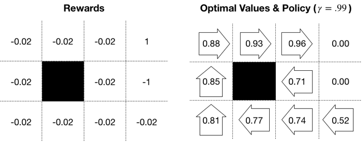
Figure 22.4: 3×4 gridworld rewards, value function, and optimal policy
Setting up the gridworld
We will begin by defining the environment parameters:
grid_size = (3, 4)
blocked_cell = (1, 1)
baseline_reward = -0.02
absorbing_cells = {(0, 3): 1, (1, 3): -1}
actions = ['L', 'U', 'R', 'D']
num_actions = len(actions)
probs = [.1, .8, .1, 0]
We will frequently need to convert between 1D and 2D representations, so we will define two helper functions for this purpose; states are one-dimensional, and cells are the corresponding 2D coordinates:
to_1d = lambda x: np.ravel_multi_index(x, grid_size)
to_2d = lambda x: np.unravel_index(x, grid_size)
Furthermore, we will precompute some data points to make the code more concise:
num_states = np.product(grid_size)
cells = list(np.ndindex(grid_size))
states = list(range(len(cells)))
cell_state = dict(zip(cells, states))
state_cell= dict(zip(states, cells))
absorbing_states = {to_1d(s):r for s, r in absorbing_cells.items()}
blocked_state = to_1d(blocked_cell)
We store the rewards for each state:
state_rewards = np.full(num_states, baseline_reward)
state_rewards[blocked_state] = 0
for state, reward in absorbing_states.items():
    state_rewards[state] = reward
state_rewards
array([-0.02, -0.02, -0.02,  1.  , -0.02,  0.  , -0.02, -1.  , -0.02,
       -0.02, -0.02, -0.02])
To account for the probabilistic environment, we also need to compute the probability distribution over the actual move for a given action:
action_outcomes = {}
for i, action in enumerate(actions):
    probs_ = dict(zip([actions[j % 4] for j in range(i,
                                               num_actions + i)], probs))
    action_outcomes[actions[(i + 1) % 4]] = probs_
Action_outcomes
{'U': {'L': 0.1, 'U': 0.8, 'R': 0.1, 'D': 0},
 'R': {'U': 0.1, 'R': 0.8, 'D': 0.1, 'L': 0},
 'D': {'R': 0.1, 'D': 0.8, 'L': 0.1, 'U': 0},
 'L': {'D': 0.1, 'L': 0.8, 'U': 0.1, 'R': 0}}
Now, we are ready to compute the transition matrix, which is the key input to the MDP.
Computing the transition matrix
The transition matrix defines the probability of ending up in a certain state S for each previous state and action A  . We will demonstrate
 pymdptoolbox and use one of the formats available to specify transitions and rewards. For both transition probabilities, we will create a NumPy array with dimensions  .
.
We first compute the target cell for each starting cell and move:
def get_new_cell(state, move):
    cell = to_2d(state)
    if actions[move] == 'U':
        return cell[0] - 1, cell[1]
    elif actions[move] == 'D':
        return cell[0] + 1, cell[1]
    elif actions[move] == 'R':
        return cell[0], cell[1] + 1
    elif actions[move] == 'L':
        return cell[0], cell[1] - 1
The following function uses the arguments starting state, action, and outcome to fill in the transition probabilities and rewards:
def update_transitions_and_rewards(state, action, outcome):
    if state in absorbing_states.keys() or state == blocked_state:
        transitions[action, state, state] = 1
    else:
        new_cell = get_new_cell(state, outcome)
        p = action_outcomes[actions[action]][actions[outcome]]
        if new_cell not in cells or new_cell == blocked_cell:
            transitions[action, state, state] += p
            rewards[action, state, state] = baseline_reward
        else:
            new_state= to_1d(new_cell)
            transitions[action, state, new_state] = p
            rewards[action, state, new_state] = state_rewards[new_state]
We generate the transition and reward values by creating placeholder data structures and iterating over the Cartesian product of  , as follows:
rewards = np.zeros(shape=(num_actions, num_states, num_states))
transitions = np.zeros((num_actions, num_states, num_states))
actions_ = list(range(num_actions))
for action, outcome, state in product(actions_, actions_, states):
    update_transitions_and_rewards(state, action, outcome)
rewards.shape, transitions.shape
((4,12,12), (4,12,12))
Implementing the value iteration algorithm
We first create the value iteration algorithm, which is slightly simpler because it implements policy evaluation and improvement in a single step. We capture the states for which we need to update the value function, excluding terminal states that have a value of 0 for lack of rewards (+1/-1 are assigned to the starting state), and skip the blocked cell:
skip_states = list(absorbing_states.keys())+[blocked_state]
states_to_update = [s for s in states if s not in skip_states]
Then, we initialize the value function and set the discount factor gamma and the convergence threshold epsilon:
V = np.random.rand(num_states)
V[skip_states] = 0
gamma = .99
epsilon = 1e-5
The algorithm updates the value function using the Bellman optimality equation, as described previously, and terminates when the L1 norm of V changes to less than epsilon in absolute terms:
while True:
    V_ = np.copy(V)
    for state in states_to_update:
        q_sa = np.sum(transitions[:, state] * (rewards[:, state] + gamma* V),
                      axis=1)
        V[state] = np.max(q_sa)
    if np.sum(np.fabs(V - V_)) < epsilon:
        break
The algorithm converges in 16 iterations and 0.0117s. It produces the following optimal value estimate, which, together with the implied optimal policy, is depicted in the right panel of Figure 22.4, earlier in this section:
pd.DataFrame(V.reshape(grid_size))
         0         1         2         3
0.884143  0.925054  0.961986  0.000000
1  0.848181  0.000000  0.714643  0.000000
2  0.808344  0.773327  0.736099  0.516082
Defining and running policy iteration
Policy iterations involve separate evaluation and improvement steps. We define the improvement part by selecting the action that maximizes the sum of the expected reward and next-state value. Note that we temporarily fill in the rewards for the terminal states to avoid ignoring actions that would lead us there:
def policy_improvement(value, transitions):
    for state, reward in absorbing_states.items():
        value[state] = reward
    return np.argmax(np.sum(transitions * value, 2),0)
We initialize the value function as before and also include a random starting policy:
pi = np.random.choice(list(range(num_actions)), size=num_states)
The algorithm alternates between policy evaluation for a greedily selected action and policy improvement until the policy stabilizes:
iterations = 0
converged = False
while not converged:
    pi_ = np.copy(pi)
    for state in states_to_update:
        action = policy[state]
        V[state] = np.dot(transitions[action, state],
                                      rewards[action, state] + gamma* V)
        pi = policy_improvement(V.copy(), transitions)
    if np.array_equal(pi_, pi):
        converged = True
    iterations += 1
Policy iteration converges after only three iterations. The policy stabilizes before the algorithm finds the optimal value function, and the optimal policy differs slightly, most notably by suggesting "up" instead of the safer "left" for the field next to the negative terminal state. This can be avoided by tightening the convergence criteria, for example, by requiring a stable policy of several rounds or by adding a threshold for the value function.
Solving MDPs using pymdptoolbox
We can also solve MDPs using the Python library pymdptoolbox, which includes a few other algorithms, including Q-learning.
To run value iteration, just instantiate the corresponding object with the desired configuration options, rewards, and transition matrices before calling the .run() method:
vi = mdp.ValueIteration(transitions=transitions,
                        reward=rewards,
                        discount=gamma,
                        epsilon=epsilon)
vi.run()
The value function estimate matches the result in the previous section:
np.allclose(V.reshape(grid_size), np.asarray(vi.V).reshape(grid_size))
Policy iteration works similarly:
pi = mdp.PolicyIteration(transitions=transitions,
                        reward=rewards,
                        discount=gamma,
                        max_iter=1000)
pi.run()
It also yields the same policy, but the value function varies by run and does not need to achieve the optimal value before the policy converges.
Lessons learned
The right panel we saw earlier in Figure 22.4 shows the optimal value estimate produced by value iteration and the corresponding greedy policy. The negative rewards, combined with the uncertainty in the environment, produce an optimal policy that involves moving away from the negative terminal state.
The results are sensitive to both the rewards and the discount factor. The cost of the negative state affects the policy in the surrounding fields, and you should modify the example in the corresponding notebook to identify threshold levels that alter the optimal action selection.
Q-learning – finding an optimal policy on the go
Q-learning was an early RL breakthrough when developed by Chris Watkins for his PhD thesis (http://www.cs.rhul.ac.uk/~chrisw/new_thesis.pdf) (1989). It introduces incremental dynamic programming to learn to control an MDP without knowing or modeling the transition and reward matrices that we used for value and policy iteration in the previous section. A convergence proof followed 3 years later (Christopher J. C. H. Watkins and Dayan 1992).
Q-learning directly optimizes the action-value function q to approximate q*. The learning proceeds "off-policy," that is, the algorithm does not need to select actions based on the policy implied by the value function alone. However, convergence requires that all state-action pairs continue to be updated throughout the training process. A straightforward way to ensure this is through an ![]() -greedy policy.
-greedy policy.
Exploration versus exploitation –  -greedy policy
An ![]() -greedy policy is a simple policy that ensures the exploration of new actions in a given state while also exploiting the learning experience . It does this by randomizing the selection of actions. An
-greedy policy is a simple policy that ensures the exploration of new actions in a given state while also exploiting the learning experience . It does this by randomizing the selection of actions. An ![]() -greedy policy selects an action randomly with a probability of
-greedy policy selects an action randomly with a probability of ![]() , and the best action according to the value function otherwise.
, and the best action according to the value function otherwise.
The Q-learning algorithm
The algorithm keeps improving a state-action value function after random initialization for a given number of episodes. At each time step, it chooses an action based on an ![]() -greedy policy, and uses a learning rate
-greedy policy, and uses a learning rate ![]() to update the value function, as follows:
to update the value function, as follows:

Note that the algorithm does not compute expected values based on the transition probabilities. Instead, it learns the Q function from the rewards Rt produced by the ![]() -greedy policy and its current estimate of the discounted value function for the next state.
-greedy policy and its current estimate of the discounted value function for the next state.
The use of the estimated value function to improve this very estimate is called bootstrapping. The Q-learning algorithm is part of the temporal difference (TD) learning algorithms. TD learning does not wait until receiving the final reward for an episode. Instead, it updates its estimates using the values of intermediate states that are closer to the final reward. In this case, the intermediate state is one time step ahead.
How to train a Q-learning agent using Python
In this section, we will demonstrate how to build a Q-learning agent using the  grid of states from the previous section. We will train the agent for 2,500 episodes, using a learning rate of
  and
and  for the
 ![]() -greedy policy (see the notebook
-greedy policy (see the notebook gridworld_q_learning.ipynb for details):
max_episodes = 2500
alpha = .1
epsilon = .05
Then, we will randomly initialize the state-action value function as a NumPy array with dimensions number of states × number of actions:
Q = np.random.rand(num_states, num_actions)
Q[skip_states] = 0
The algorithm generates 2,500 episodes that start at a random location and proceed according to the ![]() -greedy policy until termination, updating the value function according to the Q-learning rule:
-greedy policy until termination, updating the value function according to the Q-learning rule:
for episode in range(max_episodes):
    state = np.random.choice([s for s in states if s not in skip_states])
    while not state in absorbing_states.keys():
        if np.random.rand() < epsilon:
            action = np.random.choice(num_actions)
        else:
            action = np.argmax(Q[state])
        next_state = np.random.choice(states, p=transitions[action, state])
        reward = rewards[action, state, next_state]
        Q[state, action] += alpha * (reward +
                            gamma * np.max(Q[next_state])-Q[state, action])
        state = next_state
The episodes take 0.6 seconds and converge to a value function fairly close to the result of the value iteration example from the previous section. The pymdptoolbox implementation works analogously to previous examples (see the notebook for details).
Deep RL for trading with the OpenAI Gym
In the previous section, we saw how Q-learning allows us to learn the optimal state-action value function q* in an environment with discrete states and discrete actions using iterative updates based on the Bellman equation.
In this section, we will take RL one step closer to the real world and upgrade the algorithm to continuous states (while keeping actions discrete). This implies that we can no longer use a tabular solution that simply fills an array with state-action values. Instead, we will see how to approximate q* using a neural network (NN), which results in a deep Q-network. We will first discuss how deep learning integrates with RL before presenting the deep Q-learning algorithm, as well as various refinements that accelerate its convergence and make it more robust.
Continuous states also imply a more complex environment. We will demonstrate how to work with OpenAI Gym, a toolkit for designing and comparing RL algorithms. First, we'll illustrate the workflow by training a deep Q-learning agent to navigate a toy spaceship in the Lunar Lander environment. Then, we'll proceed to customize OpenAI Gym to design an environment that simulates a trading context where an agent can buy and sell a stock while competing against the market.
Value function approximation with neural networks
Continuous state and/or action spaces imply an infinite number of transitions that make it impossible to tabulate the state-action values, as in the previous section. Rather, we approximate the Q function by learning a continuous, parameterized mapping from training samples.
Motivated by the success of NNs in other domains, which we discussed in the previous chapters in Part 4, deep NNs have also become popular for approximating value functions. However, machine learning in the RL context, where the data is generated by the interaction of the model with the environment using a (possibly randomized) policy, faces distinct challenges:
- With continuous states, the agent will fail to visit most states and thus needs to generalize.
- Whereas supervised learning aims to generalize from a sample of independently and identically distributed samples that are representative and correctly labeled, in the RL context, there is only one sample per time step, so learning needs to occur online.
- Furthermore, samples can be highly correlated when sequential states are similar and the behavior distribution over states and actions is not stationary, but rather changes as a result of the agent's learning.
We will look at several techniques that have been developed to address these additional challenges.
The Deep Q-learning algorithm and extensions
Deep Q-learning estimates the value of the available actions for a given state using a deep neural network. DeepMind introduced this technique in Playing Atari with Deep Reinforcement Learning (Mnih et al. 2013), where agents learned to play games solely from pixel input.
The Deep Q-learning algorithm approximates the action-value function q by learning a set of weights ![]() of a multilayered deep Q-network (DQN) that maps states to actions so that
of a multilayered deep Q-network (DQN) that maps states to actions so that  .
.
The algorithm applies gradient descent based on a loss function that computes the squared difference between the DQN's estimate of the target:

and its estimate of the action-value of the current state-action pair  to learn the network parameters:

Both the target and the current estimate depend on the DQN weights, underlining the distinction from supervised learning where targets are fixed prior to training.
Rather than computing the full gradient, the Q-learning algorithm uses stochastic gradient descent (SGD) and updates the weights ![]() after each time step i. To explore the state-action space, the agent uses an
after each time step i. To explore the state-action space, the agent uses an ![]() -greedy policy that selects a random action with probability
-greedy policy that selects a random action with probability ![]() and follows a greedy policy that selects the action with the highest predicted q-value otherwise.
and follows a greedy policy that selects the action with the highest predicted q-value otherwise.
The basic DQN architecture has been refined in several directions to make the learning process more efficient and improve the final result; Hessel et al. (2017) combined these innovations in the Rainbow agent and demonstrated how each contributes to significantly higher performance across the Atari benchmarks. The following subsections summarize some of these innovations.
(Prioritized) Experience replay – focusing on past mistakes
Experience replay stores a history of the state, action, reward, and next state transitions experienced by the agent. It randomly samples mini-batches from this experience to update the network weights at each time step before the agent selects an ε-greedy action.
Experience replay increases sample efficiency, reduces the autocorrelation of samples collected during online learning, and limits the feedback due to current weights producing training samples that can lead to local minima or divergence (Lin and Mitchell 1992).
This technique was later refined to prioritize experience that is more important from a learning perspective. Schaul et al. (2015) approximated the value of a transition by the size of the TD error that captures how "surprising" the event was for the agent. In practice, it samples historical state transitions using their associated TD error rather than uniform probabilities.
The target network – decorrelating the learning process
To further weaken the feedback loop from the current network parameters on the NN weight updates, the algorithm was extended by DeepMind in Human-level control through deep reinforcement learning (Mnih et al. 2015) to use a slowly-changing target network.
The target network has the same architecture as the Q-network, but its weights  are only updated periodically after
 ![]() steps when they are copied from the Q-network and held constant otherwise. The target network generates the TD target predictions, that is, it takes the place of the Q-network to estimate:
steps when they are copied from the Q-network and held constant otherwise. The target network generates the TD target predictions, that is, it takes the place of the Q-network to estimate:

Double deep Q-learning – decoupling action and prediction
Q-learning has been shown to overestimate the action values because it purposely samples maximal estimated action values.
This bias can negatively affect the learning process and the resulting policy if it does not apply uniformly and alters action preferences, as shown in Deep Reinforcement Learning with Double Q-learning (van Hasselt, Guez, and Silver 2015).
To decouple the estimation of action values from the selection of actions, the Double DQN (DDQN) algorithm uses the weights ![]() of one network to select the best action given the next state, as well as the weights
of one network to select the best action given the next state, as well as the weights ![]() of another network, to provide the corresponding action value estimate:
of another network, to provide the corresponding action value estimate:
 .
. One option is to randomly select one of two identical networks for training at each iteration so that their weights will differ. A more efficient alternative is to rely on the target network to provide ![]() instead.
instead.
Introducing the OpenAI Gym
OpenAI Gym is an RL platform that provides standardized environments to test and benchmark RL algorithms using Python. It is also possible to extend the platform and register custom environments.
The Lunar Lander v2 (LL) environment requires the agent to control its motion in two dimensions based on a discrete action space and low-dimensional state observations that include position, orientation, and velocity. At each time step, the environment provides an observation of the new state and a positive or negative reward. Each episode consists of up to 1,000 time steps. Figure 22.5 shows selected frames from a successful landing after 250 episodes by the agent we will train later:

Figure 22.5: RL agent's behavior during the Lunar Lander episode
More specifically, the agent observes eight aspects of the state, including six continuous and two discrete elements. Based on the observed elements, the agent knows its location, direction, and speed of movement and whether it has (partially) landed. However, it does not know in which direction it should move, nor can it observe the inner state of the environment to understand the rules that govern its motion.
At each time step, the agent controls its motion using one of four discrete actions. It can do nothing (and continue on its current path), fire its main engine (to reduce downward motion), or steer toward the left or right using the respective orientation engines. There are no fuel limitations.
The goal is to land the agent between two flags on a landing pad at coordinates (0, 0), but landing outside of the pad is possible. The agent accumulates rewards in the range of 100-140 for moving toward the pad, depending on the exact landing spot. However, a move away from the target negates the reward the agent would have gained by moving toward the pad. Ground contact by each leg adds 10 points, while using the main engine costs -0.3 points.
An episode terminates if the agent lands or crashes, adding or subtracting 100 points, respectively, or after 1,000 time steps. Solving LL requires achieving a cumulative reward of at least 200 on average over 100 consecutive episodes.
How to implement DDQN using TensorFlow 2
The notebook 03_lunar_lander_deep_q_learning implements a DDQN agent using TensorFlow 2 that learns to solve OpenAI Gym's Lunar Lander 2.0 (LL) environment. The notebook 03_lunar_lander_deep_q_learning contains a TensorFlow 1 implementation that was discussed in the first edition and runs significantly faster because it does not rely on eager execution and also converges sooner. This section highlights key elements of the implementation; please see the notebook for much more extensive details.
Creating the DDQN agent
We create our DDQNAgent as a Python class to integrate the learning and execution logic with the key configuration parameters and performance tracking.
The agent's __init__() method takes, as arguments, information on:
- The environment characteristics, like the number of dimensions for the state observations and the number of actions available to the agent.
- The decay of the randomized exploration for the ε-greedy policy.
- The neural network architecture and the parameters for training and target network updates.
class DDQNAgent:
    def __init__(self, state_dim, num_actions, gamma,
                 epsilon_start, epsilon_end, epsilon_decay_steps,
                 epsilon_exp_decay,replay_capacity, learning_rate,
                 architecture, l2_reg, tau, batch_size,
                 log_dir='results'):
Adapting the DDQN architecture to the Lunar Lander
The DDQN architecture was first applied to the Atari domain with high-dimensional image observations and relied on convolutional layers. The LL's lower-dimensional state representation makes fully connected layers a better choice (see Chapter 17, Deep Learning for Trading).
More specifically, the network maps eight inputs to four outputs, representing the Q values for each action, so that it only takes a single forward pass to compute the action values. The DQN is trained on the previous loss function using the Adam optimizer. The agent's DQN uses three densely connected layers with 256 units each and L2 activity regularization. Using a GPU via the TensorFlow Docker image can significantly speed up NN training performance (see Chapter 17 and Chapter 18, CNNs for Financial Time Series and Satellite Images).
The DDQNAgent class's build_model() method creates the primary online and slow-moving target networks based on the architecture parameter, which specifies the number of layers and their number of units.
We set trainable to True for the primary online network and to False for the target network. This is because we simply periodically copy the online NN weights to update the target network:
    def build_model(self, trainable=True):
        layers = []
        for i, units in enumerate(self.architecture, 1):
            layers.append(Dense(units=units,
                                input_dim=self.state_dim if i == 1 else None,
                                activation='relu',
                                kernel_regularizer=l2(self.l2_reg),
                                trainable=trainable))
        layers.append(Dense(units=self.num_actions,
                            trainable=trainable))
        model = Sequential(layers)
        model.compile(loss='mean_squared_error',
                      optimizer=Adam(lr=self.learning_rate))
        return model
Memorizing transitions and replaying the experience
To enable experience replay, the agent memorizes each state transition so it can randomly sample a mini-batch during training. The memorize_transition() method receives the observation on the current and next state provided by the environment, as well as the agent's action, the reward, and a flag that indicates whether the episode is completed.
It tracks the reward history and length of each episode, applies exponential decay to epsilon at the end of each period, and stores the state transition information in a buffer:
    def memorize_transition(self, s, a, r, s_prime, not_done):
        if not_done:
            self.episode_reward += r
            self.episode_length += 1
        else:
            self.episodes += 1
            self.rewards_history.append(self.episode_reward)
            self.steps_per_episode.append(self.episode_length)
            self.episode_reward, self.episode_length = 0, 0
        self.experience.append((s, a, r, s_prime, not_done))
The replay of the memorized experience begins as soon as there are enough samples to create a full batch. The experience_replay() method predicts the Q values for the next states using the online network and selects the best action. It then selects the predicted q values for these actions from the target network to arrive at the TD targets.
Next, it trains the primary network using a single batch of current state observations as input, the TD targets as the outcome, and the mean-squared error as the loss function. Finally, it updates the target network weights every ![]() steps:
steps:
    def experience_replay(self):
        if self.batch_size > len(self.experience):
            return
        # sample minibatch from experience
        minibatch = map(np.array, zip(*sample(self.experience,
                                              self.batch_size)))
        states, actions, rewards, next_states, not_done = minibatch
        # predict next Q values to select best action
        next_q_values = self.online_network.predict_on_batch(next_states)
        best_actions = tf.argmax(next_q_values, axis=1)
        # predict the TD target
        next_q_values_target = self.target_network.predict_on_batch(
            next_states)
        target_q_values = tf.gather_nd(next_q_values_target,
                                       tf.stack((self.idx, tf.cast(
                                          best_actions, tf.int32)), axis=1))
        targets = rewards + not_done * self.gamma * target_q_values
        # predict q values
        q_values = self.online_network.predict_on_batch(states)
        q_values[[self.idx, actions]] = targets
        # train model
        loss = self.online_network.train_on_batch(x=states, y=q_values)
        self.losses.append(loss)
        if self.total_steps % self.tau == 0:
            self.update_target()
    def update_target(self):
        self.target_network.set_weights(self.online_network.get_weights())
The notebook contains additional implementation details for the ε-greedy policy and the target network weight updates.
Setting up the OpenAI environment
We will begin by instantiating and extracting key parameters from the LL environment:
env = gym.make('LunarLander-v2')
state_dim = env.observation_space.shape[0]  # number of dimensions in state
num_actions = env.action_space.n  # number of actions
max_episode_steps = env.spec.max_episode_steps  # max number of steps per episode
env.seed(42)
We will also use the built-in wrappers that permit the periodic storing of videos that display the agent's performance:
from gym import wrappers
env = wrappers.Monitor(env,
                       directory=monitor_path.as_posix(),
                       video_callable=lambda count: count % video_freq == 0,
                      force=True)
When running on a server or Docker container without a display, you can use pyvirtualdisplay.
Key hyperparameter choices
The agent's performance is quite sensitive to several hyperparameters. We will start with the discount and learning rates:
gamma=.99,  # discount factor
learning_rate=1e-4  # learning rate
We will update the target network every 100 time steps, store up to 1 million past episodes in the replay memory, and sample mini-batches of 1,024 from memory to train the agent:
tau=100  # target network update frequency
replay_capacity=int(1e6)
batch_size = 1024
The ε-greedy policy starts with pure exploration at  , linear decay to 0.01 over 250 episodes, and exponential decay thereafter:
epsilon_start=1.0
epsilon_end=0.01
epsilon_linear_steps=250
epsilon_exp_decay=0.99
The notebook contains the training loop, including experience replay, SGD, and slow target network updates.
Lunar Lander learning performance
The preceding hyperparameter settings enable the agent to solve the environment in around 300 episodes using the TensorFlow 1 implementation.
The left panel of Figure 22.6 shows the episode rewards and their moving average over 100 periods. The right panel shows the decay of exploration and the number of steps per episode. There is a stretch of some 100 episodes that often take 1,000 time steps each while the agent reduces exploration and "learns how to fly" before starting to land fairly consistently:

Figure 22.6: The DDQN agent's performance in the Lunar Lander environment
Creating a simple trading agent
In this and the following sections, we will adapt the deep RL approach to design an agent that learns how to trade a single asset. To train the agent, we will set up a simple environment with a limited set of actions, a relatively low-dimensional state with continuous observations, and other parameters.
More specifically, the environment samples a stock price time series for a single ticker using a random start date to simulate a trading period that, by default, contains 252 days or 1 year. Each state observation provides the agent with the historical returns for various lags and some technical indicators, like the relative strength index (RSI).
The agent can choose from three actions:
- Buy: Invest all capital for a long position in the stock.
- Flat: Hold cash only.
- Sell short: Take a short position equal to the amount of capital.
The environment accounts for trading cost, set to 10 basis points by default, and deducts one basis point per period without trades. The reward of the agent consists of the daily return minus trading costs.
The environment tracks the net asset value (NAV) of the agent's portfolio (consisting of a single stock) and compares it against the market portfolio, which trades frictionless to raise the bar for the agent.
An episode begins with a starting NAV of 1 unit of cash:
- If the NAV drops to 0, the episode ends with a loss.
- If the NAV hits 2.0, the agent wins.
This setting limits complexity as it focuses on a single stock and abstracts from position sizing to avoid the need for continuous actions or a larger number of discrete actions, as well as more sophisticated bookkeeping. However, it is useful to demonstrate how to customize an environment and permits for extensions.
How to design a custom OpenAI trading environment
To build an agent that learns how to trade, we need to create a market environment that provides price and other information, offers relevant actions, and tracks the portfolio to reward the agent accordingly. For a description of the efforts to build a large-scale, real-world simulation environment, see Byrd, Hybinette, and Balch (2019).
OpenAI Gym allows for the design, registration, and utilization of environments that adhere to its architecture, as described in the documentation. The file trading_env.py contains the following code examples, which illustrate the process unless noted otherwise.
The trading environment consists of three classes that interact to facilitate the agent's activities. The DataSource class loads a time series, generates a few features, and provides the latest observation to the agent at each time step. TradingSimulator tracks the positions, trades and cost, and the performance. It also implements and records the results of a buy-and-hold benchmark strategy. TradingEnvironment itself orchestrates the process. We will briefly describe each in turn; see the script for implementation details.
Designing a DataSource class
First, we code up a DataSource class to load and preprocess historical stock data to create the information used for state observations and rewards. In this example, we will keep it very simple and provide the agent with historical data on a single stock. Alternatively, you could combine many stocks into a single time series, for example, to train the agent on trading the S&P 500 constituents.
We will load the adjusted price and volume information for one ticker from the Quandl dataset, in this case for AAPL with data from the early 1980s until 2018:
class DataSource:
    """Data source for TradingEnvironment
    Loads & preprocesses daily price & volume data
    Provides data for each new episode.
    """
    def __init__(self, trading_days=252, ticker='AAPL'):
        self.ticker = ticker
        self.trading_days = trading_days
    def load_data(self):
        idx = pd.IndexSlice
        with pd.HDFStore('../data/assets.h5') as store:
            df = (store['quandl/wiki/prices']
                  .loc[idx[:, self.ticker],
                       ['adj_close', 'adj_volume', 'adj_low', 'adj_high']])
        df.columns = ['close', 'volume', 'low', 'high']
        return df
The preprocess_data() method creates several features and normalizes them. The most recent daily returns play two roles:
- An element of the observations for the current state
- The net of trading costs and, depending on the position size, the reward for the last period
The method takes the following steps, among others (refer to the Appendix for details on the technical indicators):
def preprocess_data(self):
"""calculate returns and percentiles, then removes missing values"""
   self.data['returns'] = self.data.close.pct_change()
   self.data['ret_2'] = self.data.close.pct_change(2)
   self.data['ret_5'] = self.data.close.pct_change(5)
   self.data['rsi'] = talib.STOCHRSI(self.data.close)[1]
   self.data['atr'] = talib.ATR(self.data.high,
                                self.data.low, self.data.close)
   self.data = (self.data.replace((np.inf, -np.inf), np.nan)
                .drop(['high', 'low', 'close'], axis=1)
                .dropna())
   if self.normalize:
       self.data = pd.DataFrame(scale(self.data),
                                columns=self.data.columns,
                                index=self.data.index)
The DataSource class keeps track of episode progress, provides fresh data to TradingEnvironment at each time step, and signals the end of the episodes:
def take_step(self):
    """Returns data for current trading day and done signal"""
    obs = self.data.iloc[self.offset + self.step].values
    self.step += 1
    done = self.step > self.trading_days
    return obs, done
The TradingSimulator class
The trading simulator computes the agent's reward and tracks the net asset values of the agent and "the market," which executes a buy-and-hold strategy with reinvestment. It also tracks the positions and the market return, computes trading costs, and logs the results.
The most important method of this class is the take_step method, which computes the agent's reward based on its current position, the latest stock return, and the trading costs (slightly simplified; see the script for full details):
def take_step(self, action, market_return):
    """ Calculates NAVs, trading costs and reward
        based on an action and latest market return
        returns the reward and an activity summary"""
    start_position = self.positions[max(0, self.step - 1)]
    start_nav = self.navs[max(0, self.step - 1)]
    start_market_nav = self.market_navs[max(0, self.step - 1)]
    self.market_returns[self.step] = market_return
    self.actions[self.step] = action
    end_position = action - 1 # short, neutral, long
    n_trades = end_position – start_position
    self.positions[self.step] = end_position
    self.trades[self.step] = n_trades
    time_cost = 0 if n_trades else self.time_cost_bps
    self.costs[self.step] = abs(n_trades) * self.trading_cost_bps + time_cost
    if self.step > 0:
        reward = start_position * market_return - self.costs[self.step-1]
        self.strategy_returns[self.step] = reward
        self.navs[self.step] = start_nav * (1 +
                                            self.strategy_returns[self.step])
        self.market_navs[self.step] = start_market_nav * (1 +
                                            self.market_returns[self.step])
    self.step += 1
    return reward
The TradingEnvironment class
The TradingEnvironment class subclasses gym.Env and drives the environment dynamics. It instantiates the DataSource and TradingSimulator objects and sets the action and state-space dimensionality, with the latter depending on the ranges of the features defined by DataSource:
class TradingEnvironment(gym.Env):
    """A simple trading environment for reinforcement learning.
    Provides daily observations for a stock price series
    An episode is defined as a sequence of 252 trading days with random start
    Each day is a 'step' that allows the agent to choose one of three actions.
    """
    def __init__(self, trading_days=252, trading_cost_bps=1e-3,
                 time_cost_bps=1e-4, ticker='AAPL'):
        self.data_source = DataSource(trading_days=self.trading_days,
                                      ticker=ticker)
        self.simulator = TradingSimulator(
                steps=self.trading_days,
                trading_cost_bps=self.trading_cost_bps,
                time_cost_bps=self.time_cost_bps)
        self.action_space = spaces.Discrete(3)
        self.observation_space = spaces.Box(self.data_source.min_values,
                                            self.data_source.max_values)
The two key methods of TradingEnvironment are .reset() and .step(). The former initializes the DataSource and TradingSimulator instances, as follows:
def reset(self):
    """Resets DataSource and TradingSimulator; returns first observation"""
    self.data_source.reset()
    self.simulator.reset()
    return self.data_source.take_step()[0]
Each time step relies on DataSource and TradingSimulator to provide a state observation and reward the most recent action:
def step(self, action):
    """Returns state observation, reward, done and info"""
    assert self.action_space.contains(action),
      '{} {} invalid'.format(action, type(action))
    observation, done = self.data_source.take_step()
    reward, info = self.simulator.take_step(action=action,
                                            market_return=observation[0])
    return observation, reward, done, info
Registering and parameterizing the custom environment
Before using the custom environment, just as for the Lunar Lander environment, we need to register it with the gym package, provide information about the entry_point in terms of module and class, and define the maximum number of steps per episode (the following steps occur in the q_learning_for_trading notebook):
from gym.envs.registration import register
register(
        id='trading-v0',
        entry_point='trading_env:TradingEnvironment',
        max_episode_steps=252)
We can instantiate the environment using the desired trading costs and ticker:
trading_environment = gym.make('trading-v0')
trading_environment.env.trading_cost_bps = 1e-3
trading_environment.env.time_cost_bps = 1e-4
trading_environment.env.ticker = 'AAPL'
trading_environment.seed(42)
Deep Q-learning on the stock market
The notebook q_learning_for_trading contains the DDQN agent training code; we will only highlight noteworthy differences from the previous example.
Adapting and training the DDQN agent
We will use the same DDQN agent but simplify the NN architecture to two layers of 64 units each and add dropout for regularization. The online network has 5,059 trainable parameters:
Layer (type)                 Output Shape              Param #
Dense_1 (Dense)              (None, 64)                704
Dense_2 (Dense)              (None, 64)                4160
dropout (Dropout)            (None, 64)                0
Output (Dense)               (None, 3)                 195
Total params: 5,059
Trainable params: 5,059
The training loop interacts with the custom environment in a manner very similar to the Lunar Lander case. While the episode is active, the agent takes the action recommended by its current policy and trains the online network using experience replay after memorizing the current transition. The following code highlights the key steps:
for episode in range(1, max_episodes + 1):
    this_state = trading_environment.reset()
    for episode_step in range(max_episode_steps):
        action = ddqn.epsilon_greedy_policy(this_state.reshape(-1,
                                                               state_dim))
        next_state, reward, done, _ = trading_environment.step(action)

        ddqn.memorize_transition(this_state, action,
                                 reward, next_state,
                                 0.0 if done else 1.0)
        ddqn.experience_replay()
        if done:
            break
        this_state = next_state
trading_environment.close()
We let exploration continue for 2,000 1-year trading episodes, corresponding to about 500,000 time steps; we use linear decay of ε from 1.0 to 0.1 over 500 periods with exponential decay at a factor of 0.995 thereafter.
Benchmarking DDQN agent performance
To compare the DDQN agent's performance, we not only track the buy-and-hold strategy but also generate the performance of a random agent.
Figure 22.7 shows the rolling averages over the last 100 episodes of three cumulative return values for the 2,000 training periods (left panel), as well as the share of the last 100 episodes when the agent outperformed the buy-and-hold period (right panel). It uses AAPL stock data, for which there are some 9,000 daily price and volume observations:

Figure 22.7: Trading agent performance relative to the market
This shows how the agent's performance improves steadily after 500 episodes, from the level of a random agent, and starts to outperform the buy-and-hold strategy toward the end of the experiment more than half of the time.
Lessons learned
This relatively simple agent uses no information beyond the latest market data and the reward signal compared to the machine learning models we covered elsewhere in this book. Nonetheless, it learns to make a profit and achieve performance similar to that of the market (after training on 2,000 years' worth of data, which takes only a fraction of the time on a GPU).
Keep in mind that using a single stock also increases the risk of overfitting to the data—by a lot. You can test your trained agent on new data using the saved model (see the notebook for Lunar Lander).
In summary, we have demonstrated the mechanics of setting up an RL trading environment and experimented with a basic agent that uses a small number of technical indicators. You should try to extend both the environment and the agent, for example, to choose from several assets, size the positions, and manage risks.
Reinforcement learning is often considered the most promising approach to algorithmic trading because it most accurately models the task an investor is facing. However, our dramatically simplified examples illustrate that creating a realistic environment poses a considerable challenge. Moreover, deep reinforcement learning that has achieved impressive breakthroughs in other domains may face greater obstacles given the noisy nature of financial data, which makes it even harder to learn a value function based on delayed rewards.
Nonetheless, the substantial interest in this subject makes it likely that institutional investors are working on larger-scale experiments that may yield tangible results. An interesting complementary approach beyond the scope of this book is Inverse Reinforcement Learning, which aims to identify the reward function of an agent (for example, a human trader) given its observed behavior; see Arora and Doshi (2019) for a survey and Roa-Vicens et al. (2019) for an application on trading in the limit-order book context.
Summary
In this chapter, we introduced a different class of machine learning problems that focus on automating decisions by agents that interact with an environment. We covered the key features required to define an RL problem and various solution methods.
We saw how to frame and analyze an RL problem as a finite Markov decision problem, as well as how to compute a solution using value and policy iteration. We then moved on to more realistic situations, where the transition probabilities and rewards are unknown to the agent, and saw how Q-learning builds on the key recursive relationship defined by the Bellman optimality equation in the MDP case. We saw how to solve RL problems using Python for simple MDPs and more complex environments with Q-learning.
We then expanded our scope to continuous states and applied the Deep Q-learning algorithm to the more complex Lunar Lander environment. Finally, we designed a simple trading environment using the OpenAI Gym platform, and also demonstrated how to train an agent to learn how to make a profit while trading a single stock.
In the next and final chapter, we'll present a few conclusions and key takeaways from our journey through this book and lay out some steps for you to consider as you continue building your skills to use machine learning for trading.