
7
Linear Models – From Risk Factors to Return Forecasts
The family of linear models represents one of the most useful hypothesis classes. Many learning algorithms that are widely applied in algorithmic trading rely on linear predictors because they can be efficiently trained, are relatively robust to noisy financial data, and have strong links to the theory of finance. Linear predictors are also intuitive, easy to interpret, and often fit the data reasonably well or at least provide a good baseline.
Linear regression has been known for over 200 years, since Legendre and Gauss applied it to astronomy and began to analyze its statistical properties. Numerous extensions have since adapted the linear regression model and the baseline ordinary least squares (OLS) method to learn its parameters:
- Generalized linear models (GLM) expand the scope of applications by allowing for response variables that imply an error distribution other than the normal distribution. GLMs include the probit or logistic models for categorical response variables that appear in classification problems.
- More robust estimation methods enable statistical inference where the data violates baseline assumptions due to, for example, correlation over time or across observations. This is often the case with panel data that contains repeated observations on the same units, such as historical returns on a universe of assets.
- Shrinkage methods aim to improve the predictive performance of linear models. They use a complexity penalty that biases the coefficients learned by the model, with the goal of reducing the model's variance and improving out-of-sample predictive performance.
In practice, linear models are applied to regression and classification problems with the goals of inference and prediction. Numerous asset pricing models have been developed by academic and industry researchers that leverage linear regression. Applications include the identification of significant factors that drive asset returns for better risk and performance management, as well as the prediction of returns over various time horizons. Classification problems, on the other hand, include directional price forecasts.
In this chapter, we will cover the following topics:
- How linear regression works and which assumptions it makes
- Training and diagnosing linear regression models
- Using linear regression to predict stock returns
- Use regularization to improve predictive performance
- How logistic regression works
- Converting a regression into a classification problem
You can find the code samples for this chapter and links to additional resources in the corresponding directory of the GitHub repository. The notebooks include color versions of the images.
From inference to prediction
As the name suggests, linear regression models assume that the output is the result of a linear combination of the inputs. The model also assumes a random error that allows for each observation to deviate from the expected linear relationship. The reasons that the model does not perfectly describe the relationship between inputs and output in a deterministic way include, for example, missing variables, measurement, or data collection issues.
If we want to draw statistical conclusions about the true (but not observed) linear relationship in the population based on the regression parameters estimated from the sample, we need to add assumptions about the statistical nature of these errors. The baseline regression model makes the strong assumption that the distribution of the errors is identical across observations. It also assumes that errors are independent of each other—in other words, knowing one error does not help to forecast the next error. The assumption of independent and identically distributed (IID) errors implies that their covariance matrix is the identity matrix multiplied by a constant representing the error variance.
These assumptions guarantee that the OLS method delivers estimates that are not only unbiased but also efficient, which means that OLS estimates achieve the lowest sampling error among all linear learning algorithms. However, these assumptions are rarely met in practice.
In finance, we often encounter panel data with repeated observations on a given cross section. The attempt to estimate the systematic exposure of a universe of assets to a set of risk factors over time typically reveals correlation along the time axis, in the cross-sectional dimension, or both. Hence, alternative learning algorithms have emerged that assume error covariance matrices that are more complex than multiples of the identity matrix.
On the other hand, methods that learn biased parameters for a linear model may yield estimates with lower variance and, hence, improve their predictive performance. Shrinkage methods reduce the model's complexity by applying regularization, which adds a penalty term to the linear objective function.
This penalty is positively related to the absolute size of the coefficients so that they are shrunk relative to the baseline case. Larger coefficients imply a more complex model that reacts more strongly to variations in the inputs. When properly calibrated, the penalty can limit the growth of the model's coefficients beyond what is optimal from a bias-variance perspective.
First, we will introduce the baseline techniques for cross-section and panel data for linear models, as well as important enhancements that produce accurate estimates when key assumptions are violated. We will then illustrate these methods by estimating factor models that are ubiquitous in the development of algorithmic trading strategies. Finally, we will turn our attention to how shrinkage methods apply regularization and demonstrate how to use them to predict asset returns and generate trading signals.
The baseline model – multiple linear regression
We will begin with the model's specification and objective function, the methods we can use to learn its parameters, and the statistical assumptions that allow the inference and diagnostics of these assumptions. Then, we will present extensions that we can use to adapt the model to situations that violate these assumptions. Useful references for additional background include Wooldridge (2002 and 2008).
How to formulate the model
The multiple regression model defines a linear functional relationship between one continuous outcome variable and p input variables that can be of any type but may require preprocessing. Multivariate regression, in contrast, refers to the regression of multiple outputs on multiple input variables.
In the population, the linear regression model has the following form for a single instance of the output y, an input vector  , and the error
 ![]() :
:

The interpretation of the coefficients is straightforward: the value of a coefficient ![]() is the partial, average effect of the variable xi on the output, holding all other variables constant.
is the partial, average effect of the variable xi on the output, holding all other variables constant.
We can also write the model more compactly in matrix form. In this case, y is a vector of N output observations, X is the design matrix with N rows of observations on the p variables plus a column of 1s for the intercept, and ![]() is the vector containing the P = p+1 coefficients:
is the vector containing the P = p+1 coefficients:

The model is linear in its p +1 parameters but can represent nonlinear relationships if we choose or transform variables accordingly, for example, by including a polynomial basis expansion or logarithmic terms. You can also use categorical variables with dummy encoding, and include interactions between variables by creating new inputs of the form xixj.
To complete the formulation of the model from a statistical point of view so that we can test hypotheses about its parameters, we need to make specific assumptions about the error term. We'll do this after introducing the most important methods to learn the parameters.
How to train the model
There are several methods we can use to learn the model parameters from the data: ordinary least squares (OLS), maximum likelihood estimation (MLE), and stochastic gradient descent (SGD). We will present each method in turn.
Ordinary least squares – how to fit a hyperplane to the data
The method of least squares is the original method that learns the parameters of the hyperplane that best approximates the output from the input data. As the name suggests, it takes the best approximation to minimize the sum of the squared distances between the output value and the hyperplane represented by the model.
The difference between the model's prediction and the actual outcome for a given data point is the residual (whereas the deviation of the true model from the true output in the population is called error). Hence, in formal terms, the least-squares estimation method chooses the coefficient vector to minimize the residual sum of squares (RSS):

Thus, the least-squares coefficients  are computed as:

The optimal parameter vector that minimizes the RSS results from setting the derivatives with respect to ![]() of the preceding expression to zero. Assuming X has full column rank, which requires that the input variables are not linearly dependent, it is thus invertible, and we obtain a unique solution, as follows:
of the preceding expression to zero. Assuming X has full column rank, which requires that the input variables are not linearly dependent, it is thus invertible, and we obtain a unique solution, as follows:

When y and X have means of zero, which can be achieved by subtracting their respective means, ![]() represents the ratio of the covariance between the inputs and the outputs
represents the ratio of the covariance between the inputs and the outputs  and the output variance
There is also a geometric interpretation: the coefficients that minimize RSS ensure that the vector of residuals  is orthogonal to the subspace of
  spanned by the P columns of X, and the estimates
 ![]() are orthogonal projections into that subspace.
are orthogonal projections into that subspace.
Maximum likelihood estimation
MLE is an important general method used to estimate the parameters of a statistical model. It relies on the likelihood function, which computes how likely it is to observe the sample of outputs when given the input data as a function of the model parameters. The likelihood differs from probabilities in that it is not normalized to a range from 0 to 1.
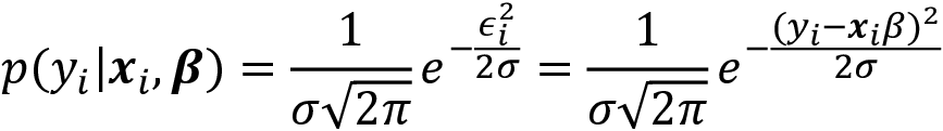
We can set up the likelihood function for the multiple linear regression example by assuming a distribution for the error term, such as the standard normal distribution:

This allows us to compute the conditional probability of observing a given output yi given the corresponding input vector xi and the parameters ![]() ,
,  :
:
Assuming the output values are conditionally independent, given the inputs, the likelihood of the sample is proportional to the product of the conditional probabilities of the individual output data points. Since it is easier to work with sums than with products, we apply the logarithm to obtain the log-likelihood function:

The goal of MLE is to choose the model parameters that maximize the probability of the observed output sample, taking the inputs as given. Hence, the MLE parameter estimate results from maximizing the log-likelihood function:

Due to the assumption of normally distributed errors, maximizing the log-likelihood function produces the same parameter solution as least squares. This is because the only expression that depends on the parameters is the squared residual in the exponent.
For other distributional assumptions and models, MLE will produce different results, as we will see in the last section on binary classification, where the outcome follows a Bernoulli distribution. Furthermore, MLE is a more general estimation method because, in many cases, the least-squares method is not applicable, as we will see later for logistic regression.
Gradient descent
Gradient descent is a general-purpose optimization algorithm that will find stationary points of smooth functions. The solution will be a global optimum if the objective function is convex. Variations of gradient descent are widely used in training complex neural networks, but also to compute solutions for MLE problems.
The algorithm uses the gradient of the objective function. The gradient contains the partial derivatives of the objective with respect to the parameters. These derivatives indicate how much the objective changes for an infinitesimal (infinitely small) step in the direction of the corresponding parameters. It turns out that the maximal change of the function value results from a step in the direction of the gradient itself.
Figure 7.1 sketches the process for a single variable x and a convex function f(x), where we are looking for the minimum, x0 . Where the function has a negative slope, gradient descent increases the target value for x0, and decreases the values otherwise:

Figure 7.1: Gradient descent
When we minimize a function that describes, for example, the cost of a prediction error, the algorithm computes the gradient for the current parameter values using the training data. Then, it modifies each parameter in proportion to the negative value of its corresponding gradient component. As a result, the objective function will assume a lower value and move the parameters closer to the solution. The optimization stops when the gradient becomes small, and the parameter values change very little.
The size of these steps is determined by the learning rate, which is a critical parameter that may require tuning. Many implementations include the option for this learning rate to gradually decrease with the number of iterations. Depending on the size of the data, the algorithm may iterate many times over the entire dataset. Each such iteration is called an epoch. The number of epochs and the tolerance used to stop further iterations are additional hyperparameters you can tune.
Stochastic gradient descent randomly selects a data point and computes the gradient for this data point, as opposed to an average over a larger sample to achieve a speedup. There are also batch versions that use a certain number of data points for each step.
The Gauss–Markov theorem
To assess the statistical properties of the model and run inference, we need to make assumptions about the residuals that represent the part of the input data the model is unable to correctly fit or "explain."
The Gauss–Markov theorem (GMT) defines the assumptions required for OLS to produce unbiased estimates of the model parameters ![]() , and for these estimates to have the lowest standard error among all linear models for cross-sectional data.
, and for these estimates to have the lowest standard error among all linear models for cross-sectional data.
The baseline multiple regression model makes the following GMT assumptions (Wooldridge 2008):
- In the population, linearity holds so that
 , where
  are unknown but constant and
  is a random error.
 - The data for the input variables
 is a random sample from the population.
 - No perfect collinearity—there are no exact linear relationships among the input variables.
- The error has a conditional mean of zero given any of the inputs:
 .
. - Homoskedasticity—the error term
 has constant variance given the inputs:
The fourth assumption implies that no missing variable exists that is correlated with any of the input variables.
Under the first four assumptions (GMT 1-4), the OLS method delivers unbiased estimates. Including an irrelevant variable does not bias the intercept and slope estimates, but omitting a relevant variable will result in biased parameter estimates.
Under GMT 1-4, OLS is then also consistent: as the sample size increases, the estimates converge to the true value as the standard errors become arbitrary. The converse is, unfortunately, also true: if the conditional expectation of the error is not zero because the model misses a relevant variable or the functional form is wrong (for example, quadratic or log terms are missing), then all parameter estimates are biased. If the error is correlated with any of the input variables, then OLS is also not consistent and adding more data will not remove the bias.
If we add the fifth assumption, then OLS also produces the best linear unbiased estimates (BLUE). Best means that the estimates have the lowest standard error among all linear estimators. Hence, if the five assumptions hold and the goal is statistical inference, then the OLS estimates are the way to go. If the goal, however, is to predict, then we will see that other estimators exist that trade some bias for a lower variance to achieve superior predictive performance in many settings.
Now that we have introduced the basic OLS assumptions, we can take a look at inference in small and large samples.
How to conduct statistical inference
Inference in the linear regression context aims to draw conclusions from the sample data about the true relationship in the population. This includes testing hypotheses about the significance of the overall relationship or the values of particular coefficients, as well as estimates of confidence intervals.
The key ingredient for statistical inference is a test statistic with a known distribution, typically computed from a quantity of interest like a regression coefficient. We can formulate a null hypothesis about this statistic and compute the probability of observing the actual value for this statistic, given the sample under the assumption that the hypothesis is correct. This probability is commonly referred to as the p-value: if it drops below a significance threshold (typically 5 percent), then we reject the hypothesis because it makes the value that we observed for the test statistic in the sample very unlikely. On the flip side, the p-value reflects the probability that we are wrong in rejecting what is, in fact, a correct hypothesis.
In addition to the five GMT assumptions, the classical linear model assumes normality—that the population error is normally distributed and independent of the input variables. This strong assumption implies that the output variable is normally distributed, conditional on the input variables. It allows for the derivation of the exact distribution of the coefficients, which, in turn, implies exact distributions of the test statistics that are needed for exact hypotheses tests in small samples. This assumption often fails in practice—asset returns, for instance, are not normally distributed.
Fortunately, however, the test statistics used under normality are also approximately valid when normality does not hold. More specifically, the following distributional characteristics of the test statistics hold approximately under GMT assumptions 1–5 and exactly when normality holds:
- The parameter estimates follow a multivariate normal distribution:
 .
. - Under GMT 1–5, the parameter estimates are unbiased, and we can get an unbiased estimate of
 , the constant error variance, using
  .
. - The t-statistic for a hypothesis test about an individual coefficient
 is
is  and follows a t distribution with N-p-1 degrees of freedom, where
  is the j's element of the diagonal of
  .
. - The t distribution converges to the normal distribution. Since the 97.5 quantile of the normal distribution is about 1.96, a useful rule of thumb for a 95 percent confidence interval around a parameter estimate is
 , where se means standard error. An interval that includes zero implies that we can't reject the null hypothesis that the true parameter is zero and, hence, irrelevant for the model.
 - The F-statistic allows for tests of restrictions on several parameters, including whether the entire regression is significant. It measures the change (reduction) in the RSS that results from additional variables.
- Finally, the Lagrange multiplier (LM) test is an alternative to the F-test for testing multiple restrictions.
How to diagnose and remedy problems
Diagnostics validate the model assumptions and help us prevent wrong conclusions when interpreting the result and conducting statistical inference. They include goodness of fit measures and various tests of the assumptions about the error term, including how closely the residuals match a normal distribution.
Furthermore, diagnostics evaluate whether the residual variance is indeed constant or exhibits heteroskedasticity (covered later in this section). They also test if the errors are conditionally uncorrelated or exhibit serial correlation, that is, if knowing one error helps to predict consecutive errors.
In addition to conducting the following diagnostic tests, you should always visually inspect the residuals. This helps to detect whether they reflect systematic patterns, as opposed to random noise that suggests the model is missing one or more factors that drive the outcome.
Goodness of fit
Goodness-of-fit measures assess how well a model explains the variation in the outcome. They help to evaluate the quality of the model specification, for instance, when selecting among different model designs.
Goodness-of-fit metrics differ in how they measure the fit. Here, we will focus on in-sample metrics; we will use out-of-sample testing and cross-validation when we focus on predictive models in the next section.
Prominent goodness-of-fit measures include the (adjusted) R2, which should be maximized and is based on the least-squares estimate:
- R2 measures the share of the variation in the outcome data explained by the model and is computed as
 , where TSS is the sum of squared deviations of the outcome from its mean. It also corresponds to the squared correlation coefficient between the actual outcome values and those estimated by the model. The implicit goal is to maximize R2. However, it never decreases as we add more variables. One of the shortcomings of R2, therefore, is that it encourages overfitting.
 - The adjusted R2 penalizes R2 for adding more variables; each additional variable needs to reduce the RSS significantly to produce better goodness of fit.
Alternatively, the Akaike information criterion (AIC) and the Bayesian information criterion (BIC) are to be minimized and are based on the maximum-likelihood estimate:
 , where
  is the value of the maximized likelihood function and k is the number of parameters.
 , where N is the sample size.
Both metrics penalize for complexity. BIC imposes a higher penalty, so it might underfit relative to AIC and vice versa.
Conceptually, AIC aims to find the model that best describes an unknown data-generating process, whereas BIC tries to find the best model among the set of candidates. In practice, both criteria can be used jointly to guide model selection when the goal is an in-sample fit; otherwise, cross-validation and selection based on estimates of generalization error are preferable.
Heteroskedasticity
GMT assumption 5 requires the residual covariance to take the shape  , that is, a diagonal matrix with entries equal to the constant variance of the error term. Heteroskedasticity occurs when the residual variance is not constant but differs across observations. If the residual variance is positively correlated with an input variable, that is, when errors are larger for input values that are far from their mean, then OLS standard error estimates will be too low; consequently, the t-statistic will be inflated, leading to false discoveries of relationships where none actually exist.
Diagnostics starts with a visual inspection of the residuals. Systematic patterns in the (supposedly random) residuals suggest statistical tests of the null hypothesis that errors are homoscedastic against various alternatives. These tests include the Breusch–Pagan and White tests.
There are several ways to correct OLS estimates for heteroskedasticity:
- Robust standard errors (sometimes called White standard errors) take heteroskedasticity into account when computing the error variance using a so-called sandwich estimator.
- Clustered standard errors assume that there are distinct groups in your data that are homoscedastic, but the error variance differs between groups. These groups could be different asset classes or equities from different industries.
Several alternatives to OLS estimate the error covariance matrix using different assumptions when  . The following are available in
 statsmodels:
- Weighted least squares (WLS): For heteroskedastic errors where the covariance matrix has only diagonal entries, as for OLS, but now the entries are allowed to vary.
- Feasible generalized least squares (GLSAR): For autocorrelated errors that follow an autoregressive AR(p) process (see Chapter 9, Time-Series Models for Volatility Forecasts and Statistical Arbitrage).
- Generalized least squares (GLS): For arbitrary covariance matrix structure; yields efficient and unbiased estimates in the presence of heteroskedasticity or serial correlation.
Serial correlation
Serial correlation means that consecutive residuals produced by linear regression are correlated, which violates the fourth GMT assumption. Positive serial correlation implies that the standard errors are underestimated and that the t-statistics will be inflated, leading to false discoveries if ignored. However, there are procedures to correct for serial correlation when calculating standard errors.
The Durbin–Watson statistic diagnoses serial correlation. It tests the hypothesis that the OLS residuals are not autocorrelated against the alternative that they follow an autoregressive process (which we will explore in the next chapter). The test statistic ranges from 0 to 4; values near 2 indicate non-autocorrelation, lower values suggest positive autocorrelation, and higher values indicate negative autocorrelation. The exact threshold values depend on the number of parameters and observations and need to be looked up in tables.
Multicollinearity
Multicollinearity occurs when two or more independent variables are highly correlated. This poses several challenges:
- It is difficult to determine which factors influence the dependent variable.
- The individual p-values can be misleading—a p-value can be high, even if the variable is, in fact, important.
- The confidence intervals for the regression coefficients will be too wide, possibly even including zero. This complicates the determination of an independent variable's effect on the outcome.
There is no formal or theory-based solution that corrects for multicollinearity. Instead, try to remove one or more of the correlated input variables, or increase the sample size.
How to run linear regression in practice
The accompanying notebook, linear_regression_intro.ipynb, illustrates a simple and then a multiple linear regression, the latter using both OLS and gradient descent. For the multiple regression, we generate two random input variables x1 and x2 that range from -50 to +50, and an outcome variable that's calculated as a linear combination of the inputs, plus random Gaussian noise, to meet the normality assumption GMT 6:

OLS with statsmodels
We use statsmodels to estimate a multiple regression model that accurately reflects the data-generating process, as follows:
import statsmodels.api as sm
X_ols = sm.add_constant(X)
model = sm.OLS(y, X_ols).fit()
model.summary()
This yields the following OLS Regression Results summary:

Figure 7.2: OLS Regression Results summary
The upper part of the summary displays the dataset characteristics—namely, the estimation method and the number of observations and parameters—and indicates that standard error estimates do not account for heteroskedasticity. The middle panel shows the coefficient values that closely reflect the artificial data-generating process. We can confirm that the estimates displayed in the middle of the summary result can be obtained using the OLS formula derived previously:
beta = np.linalg.inv(X_ols.T.dot(X_ols)).dot(X_ols.T.dot(y))
pd.Series(beta, index=X_ols.columns)
const   53.29
X_1      0.99
X_2      2.96
The following code visualizes how the model fitted by the model to the randomly generated data points:
three_dee = plt.figure(figsize=(15, 5)).gca(projection='3d')
three_dee.scatter(data.X_1, data.X_2, data.Y, c='g')
data['y-hat'] = model.predict()
to_plot = data.set_index(['X_1', 'X_2']).unstack().loc[:, 'y-hat']
three_dee.plot_surface(X_1, X_2, to_plot.values, color='black', alpha=0.2, linewidth=1, antialiased=True)
for _, row in data.iterrows():
    plt.plot((row.X_1, row.X_1), (row.X_2, row.X_2), (row.Y, row['y-hat']),              'k-');
three_dee.set_xlabel('$X_1$');three_dee.set_ylabel('$X_2$');three_dee.set_zlabel('$Y, hat{Y}$')
Figure 7.3 displays the resulting hyperplane and original data points:

Figure 7.3: Regression hyperplane
The upper right part of the panel displays the goodness-of-fit measures we just discussed, alongside the F-test, which rejects the hypothesis that all coefficients are zero and irrelevant. Similarly, the t-statistics indicate that intercept and both slope coefficients are, unsurprisingly, highly significant.
The bottom part of the summary contains the residual diagnostics. The left panel displays skew and kurtosis, which are used to test the normality hypothesis. Both the Omnibus and the Jarque–Bera tests fail to reject the null hypothesis that the residuals are normally distributed. The Durbin–Watson statistic tests for serial correlation in the residuals and has a value near 2, which, given two parameters and 625 observations, fails to reject the hypothesis of no serial correlation, as outlined in the previous section on this topic.
Lastly, the condition number provides evidence about multicollinearity: it is the ratio of the square roots of the largest and the smallest eigenvalue of the design matrix that contains the input data. A value above 30 suggests that the regression may have significant multicollinearity.
statsmodels includes additional diagnostic tests that are linked in the notebook.
Stochastic gradient descent with sklearn
The sklearn library includes an SGDRegressor model in its linear_models module. To learn the parameters for the same model using this method, we need to standardize the data because the gradient is sensitive to the scale.
We use the StandardScaler() for this purpose: it computes the mean and the standard deviation for each input variable during the fit step, and then subtracts the mean and divides by the standard deviation during the transform step, which we can conveniently conduct in a single fit_transform() command:
scaler = StandardScaler()
X_ = scaler.fit_transform(X)
Then, we instantiate SGDRegressor using the default values except for a random_state setting to facilitate replication:
sgd = SGDRegressor(loss='squared_loss',
                   fit_intercept=True,
                   shuffle=True, # shuffle data for better estimates
                   random_state=42,
                   learning_rate='invscaling', # reduce rate over time
                   eta0=0.01, # parameters for learning rate path
                   power_t=0.25)
Now, we can fit the sgd model, create the in-sample predictions for both the OLS and the sgd models, and compute the root mean squared error for each:
sgd.fit(X=X_, y=y)
resids = pd.DataFrame({'sgd': y - sgd.predict(X_),
                      'ols': y - model.predict(sm.add_constant(X))})
resids.pow(2).sum().div(len(y)).pow(.5)
ols   48.22
sgd   48.22
As expected, both models yield the same result. We will now take on a more ambitious project using linear regression to estimate a multi-factor asset pricing model.
How to build a linear factor model
Algorithmic trading strategies use factor models to quantify the relationship between the return of an asset and the sources of risk that are the main drivers of these returns. Each factor risk carries a premium, and the total asset return can be expected to correspond to a weighted average of these risk premia.
There are several practical applications of factor models across the portfolio management process, from construction and asset selection to risk management and performance evaluation. The importance of factor models continues to grow as common risk factors are now tradeable:
- A summary of the returns of many assets, by a much smaller number of factors, reduces the amount of data required to estimate the covariance matrix when optimizing a portfolio.
- An estimate of the exposure of an asset or a portfolio to these factors allows for the management of the resulting risk, for instance, by entering suitable hedges when risk factors are themselves traded or can be proxied.
- A factor model also permits the assessment of the incremental signal content of new alpha factors.
- A factor model can also help assess whether a manager's performance, relative to a benchmark, is indeed due to skillful asset selection and market timing, or if the performance can instead be explained by portfolio tilts toward known return drivers. These drivers can, today, be replicated as low-cost, passively managed funds that do not incur active management fees.
The following examples apply to equities, but risk factors have been identified for all asset classes (Ang 2014).
From the CAPM to the Fama–French factor models
Risk factors have been a key ingredient to quantitative models since the capital asset pricing model (CAPM) explained the expected returns of all N assets  using their respective exposure
 ![]() to a single factor, the expected excess return of the overall market over the risk-free rate
to a single factor, the expected excess return of the overall market over the risk-free rate ![]() . The CAPM model takes the following linear form:
. The CAPM model takes the following linear form:

This differs from the classic fundamental analysis, à la Dodd and Graham, where returns depend on firm characteristics. The rationale is that, in the aggregate, investors cannot eliminate this so-called systematic risk through diversification. Hence, in equilibrium, they require compensation for holding an asset commensurate with its systematic risk. The model implies that, given efficient markets where prices immediately reflect all public information, there should be no superior risk-adjusted returns. In other words, the value of ![]() should be zero.
should be zero.
Empirical tests of the model use linear regression and have consistently failed, for example, by identifying anomalies in the form of superior risk-adjusted returns that do not depend on overall market exposure, such as higher returns for smaller firms (Goyal 2012).
These failures have prompted a lively debate about whether the efficient markets or the single factor aspect of the joint hypothesis is to blame. It turns out that both premises are probably wrong:
- Joseph Stiglitz earned the 2001 Nobel Prize in economics in part for showing that markets are generally not perfectly efficient: if markets are efficient, there is no value in collecting data because this information is already reflected in prices. However, if there is no incentive to gather information, it is hard to see how it should be already reflected in prices.
- On the other hand, theoretical and empirical improvements of the CAPM suggest that additional factors help explain some of the anomalies mentioned previously, which result in various multi-factor models.
Stephen Ross proposed the arbitrage pricing theory (APT) in 1976 as an alternative that allows for several risk factors while eschewing market efficiency. In contrast to the CAPM, it assumes that opportunities for superior returns due to mispricing may exist but will quickly be arbitraged away. The theory does not specify the factors, but research suggests that the most important are changes in inflation and industrial production, as well as changes in risk premia or the term structure of interest rates.
Kenneth French and Eugene Fama (who won the 2013 Nobel Prize) identified additional risk factors that depend on firm characteristics and are widely used today. In 1993, the Fama–French three-factor model added the relative size and value of firms to the single CAPM source of risk. In 2015, the five-factor model further expanded the set to include firm profitability and level of investment, which had been shown to be significant in the intervening years. In addition, many factor models include a price momentum factor.
The Fama–French risk factors are computed as the return difference on diversified portfolios with high or low values, according to metrics that reflect a given risk factor. These returns are obtained by sorting stocks according to these metrics and then going long stocks above a certain percentile, while shorting stocks below a certain percentile. The metrics associated with the risk factors are defined as follows:
- Size: Market equity (ME)
- Value: Book value of equity (BE) divided by ME
- Operating profitability (OP): Revenue minus cost of goods sold/assets
- Investment: Investment/assets
There are also unsupervised learning techniques for the data-driven discovery of risk factors that use factors and principal component analysis. We will explore this in Chapter 13, Data-Driven Risk Factors and Asset Allocation with Unsupervised Learning.
Obtaining the risk factors
Fama and French make updated risk factors and research portfolio data available through their website, and you can use the pandas_datareader library to obtain the data. For this application, refer to the fama_macbeth.ipynb notebook for the following code examples and additional detail.
In particular, we will be using the five Fama–French factors that result from sorting stocks, first into three size groups and then into two, for each of the remaining three firm-specific factors. Hence, the factors involve three sets of value-weighted portfolios formed as  sorts on size and book-to-market, size and operating profitability, and size and investment. The risk factor values computed as the average returns of the portfolios (PF) are outlined in the following table:
|
Concept |
Label |
Name |
Risk factor calculation |
|
Size |
SMB |
Small minus big |
Nine small stock PF minus nine large stock PF. |
|
Value |
HML |
High minus low |
Two value PF minus two growth (with low BE/ME value) PF. |
|
Profitability |
RMW |
Robust minus weak |
Two robust OP PF minus two weak OP PF. |
|
Investment |
CMA |
Conservative minus aggressive |
Two conservative investment portfolios, minus two aggressive investment portfolios. |
|
Market |
Rm-Rf |
Excess return on the market |
Value-weight return of all firms incorporated in and listed on major US exchanges with good data, minus the one-month Treasury bill rate. |
We will use returns at a monthly frequency that we will obtain for the period 2010–2017, as follows:
import pandas_datareader.data as web
ff_factor = 'F-F_Research_Data_5_Factors_2x3'
ff_factor_data = web.DataReader(ff_factor, 'famafrench', start='2010',
                               end='2017-12')[0]
ff_factor_data.info()
PeriodIndex: 96 entries, 2010-01 to 2017-12
Freq: M
Data columns (total 6 columns):
Mkt-RF 96 non-null float64
SMB    96 non-null float64
HML    96 non-null float64
RMW    96 non-null float64
CMA    96 non-null float64
RF     96 non-null float64
Fama and French also made numerous portfolios available that we can use to illustrate the estimation of the factor exposures, as well as the value of the risk premia available in the market for a given time period. We will use a panel of the 17 industry portfolios at a monthly frequency. We will subtract the risk-free rate from the returns because the factor model works with excess returns:
ff_portfolio = '17_Industry_Portfolios'
ff_portfolio_data = web.DataReader(ff_portfolio, 'famafrench', start='2010',
                                  end='2017-12')[0]
ff_portfolio_data = ff_portfolio_data.sub(ff_factor_data.RF, axis=0)
ff_factor_data = ff_factor_data.drop('RF', axis=1)
ff_portfolio_data.info()
PeriodIndex: 96 entries, 2010-01 to 2017-12
Freq: M
Data columns (total 17 columns):
Food     96 non-null float64
Mines    96 non-null float64
Oil      96 non-null float64
...
Rtail    96 non-null float64
Finan    96 non-null float64
Other    96 non-null float64
We will now build a linear factor model based on this panel data using a method that addresses the failure of some basic linear regression assumptions.
Fama–Macbeth regression
Given data on risk factors and portfolio returns, it is useful to estimate the portfolio's exposure to these returns to learn how much they drive the portfolio's returns. It is also of interest to understand the premium that the market pays for the exposure to a given factor, that is, how much taking this risk is worth. The risk premium then permits to estimate the return for any portfolio provide we know or can assume its factor exposure.
More formally, we will have i=1, ..., N asset or portfolio returns over t=1, ..., T periods, and each asset's excess period return will be denoted. The goal is to test whether the j=1, ..., M factors explain the excess returns and the risk premium associated with each factor. In our case, we have N=17 portfolios and M=5 factors, each with 96 periods of data.
Factor models are estimated for many stocks in a given period. Inference problems will likely arise in such cross-sectional regressions because the fundamental assumptions of classical linear regression may not hold. Potential violations include measurement errors, covariation of residuals due to heteroskedasticity and serial correlation, and multicollinearity (Fama and MacBeth 1973).
To address the inference problem caused by the correlation of the residuals, Fama and MacBeth proposed a two-step methodology for a cross-sectional regression of returns on factors. The two-stage Fama–Macbeth regression is designed to estimate the premium rewarded for the exposure to a particular risk factor by the market. The two stages consist of:
- First stage: N time-series regression, one for each asset or portfolio, of its excess returns on the factors to estimate the factor loadings. In matrix form, for each asset:

- Second stage: T cross-sectional regression, one for each time period, to estimate the risk premium. In matrix form, we obtain a vector of risk premia for each period:

Now, we can compute the factor risk premia as the time average and get a t-statistic to assess their individual significance, using the assumption that the risk premia estimates are independent over time:

If we had a very large and representative data sample on traded risk factors, we could use the sample mean as a risk premium estimate. However, we typically do not have a sufficiently long history to, and the margin of error around the sample mean could be quite large. The Fama–Macbeth methodology leverages the covariance of the factors with other assets to determine the factor premia.
The second moment of asset returns is easier to estimate than the first moment, and obtaining more granular data improves estimation considerably, which is not true of mean estimation.
We can implement the first stage to obtain the 17 factor loading estimates as follows:
betas = []
for industry in ff_portfolio_data:
    step1 = OLS(endog=ff_portfolio_data.loc[ff_factor_data.index, industry],
                exog=add_constant(ff_factor_data)).fit()
    betas.append(step1.params.drop('const'))
betas = pd.DataFrame(betas,
                     columns=ff_factor_data.columns,
                     index=ff_portfolio_data.columns)
betas.info()
Index: 17 entries, Food  to Other
Data columns (total 5 columns):
Mkt-RF    17 non-null float64
SMB       17 non-null float64
HML       17 non-null float64
RMW       17 non-null float64
CMA       17 non-null float64
For the second stage, we run 96 regressions of the period returns for the cross section of portfolios on the factor loadings:
lambdas = []
for period in ff_portfolio_data.index:
    step2 = OLS(endog=ff_portfolio_data.loc[period, betas.index],
                exog=betas).fit()
    lambdas.append(step2.params)
lambdas = pd.DataFrame(lambdas,
                       index=ff_portfolio_data.index,
                       columns=betas.columns.tolist())
lambdas.info()
PeriodIndex: 96 entries, 2010-01 to 2017-12
Freq: M
Data columns (total 5 columns):
Mkt-RF    96 non-null float64
SMB       96 non-null float64
HML       96 non-null float64
RMW       96 non-null float64
CMA       96 non-null float64
Finally, we compute the average for the 96 periods to obtain our factor risk premium estimates:
lambdas.mean()
Mkt-RF    1.243632
SMB      -0.004863
HML      -0.688167
RMW      -0.237317
CMA      -0.318075
RF       -0.013280
The linearmodels library extends statsmodels with various models for panel data and also implements the two-stage Fama–MacBeth procedure:
model = LinearFactorModel(portfolios=ff_portfolio_data,
                          factors=ff_factor_data)
res = model.fit()
This provides us with the same result:

Figure 7.4: LinearFactorModel estimation summary
The accompanying notebook illustrates the use of categorical variables by using industry dummies when estimating risk premia for a larger panel of individual stocks.
Regularizing linear regression using shrinkage
The least-squares method to train a linear regression model will produce the best linear and unbiased coefficient estimates when the Gauss–Markov assumptions are met. Variations like GLS fare similarly well, even when OLS assumptions about the error covariance matrix are violated. However, there are estimators that produce biased coefficients to reduce the variance and achieve a lower generalization error overall (Hastie, Tibshirani, and Friedman 2009).
When a linear regression model contains many correlated variables, their coefficients will be poorly determined. This is because the effect of a large positive coefficient on the RSS can be canceled by a similarly large negative coefficient on a correlated variable. As a result, the risk of prediction errors due to high variance increases because this wiggle room for the coefficients makes the model more likely to overfit to the sample.
How to hedge against overfitting
One popular technique to control overfitting is that of regularization, which involves the addition of a penalty term to the error function to discourage the coefficients from reaching large values. In other words, size constraints on the coefficients can alleviate the potentially negative impact on out-of-sample predictions. We will encounter regularization methods for all models since overfitting is such a pervasive problem.
In this section, we will introduce shrinkage methods that address two motivations to improve on the approaches to linear models discussed so far:
- Prediction accuracy: The low bias but high variance of least-squares estimates suggests that the generalization error could be reduced by shrinking or setting some coefficients to zero, thereby trading off a slightly higher bias for a reduction in the variance of the model.
- Interpretation: A large number of predictors may complicate the interpretation or communication of the big picture of the results. It may be preferable to sacrifice some detail to limit the model to a smaller subset of parameters with the strongest effects.
Shrinkage models restrict the regression coefficients by imposing a penalty on their size. They achieve this goal by adding a term  to the objective function. This term implies that the coefficients of a shrinkage model minimize the RSS, plus a penalty that is positively related to the (absolute) size of the coefficients.
The added penalty thus turns the linear regression coefficients into the solution to a constrained minimization problem that, in general, takes the following Lagrangian form:

The regularization parameter ![]() determines the size of the penalty effect, that is, the strength of the regularization. As soon as
determines the size of the penalty effect, that is, the strength of the regularization. As soon as ![]() is positive, the coefficients will differ from the unconstrained least squared parameters, which implies a biased estimate. You should choose hyperparameter
is positive, the coefficients will differ from the unconstrained least squared parameters, which implies a biased estimate. You should choose hyperparameter ![]() adaptively via cross-validation to minimize an estimate of the expected prediction error. We will illustrate how to do so in the next section.
adaptively via cross-validation to minimize an estimate of the expected prediction error. We will illustrate how to do so in the next section.
Shrinkage models differ by how they calculate the penalty, that is, the functional form of S. The most common versions are the ridge regression, which uses the sum of the squared coefficients, and the lasso model, which bases the penalty on the sum of the absolute values of the coefficients.
Elastic net regression, which is not explicitly covered here, uses a combination of both. Scikit-learn includes an implementation that works very similarly to the examples we will demonstrate here.
How ridge regression works
Ridge regression shrinks the regression coefficients by adding a penalty to the objective function that equals the sum of the squared coefficients, which in turn corresponds to the L2 norm of the coefficient vector (Hoerl and Kennard 1970):

Hence, the ridge coefficients are defined as:

The intercept ![]() has been excluded from the penalty to make the procedure independent of the origin chosen for the output variable—otherwise, adding a constant to all output values would change all slope parameters, as opposed to a parallel shift.
has been excluded from the penalty to make the procedure independent of the origin chosen for the output variable—otherwise, adding a constant to all output values would change all slope parameters, as opposed to a parallel shift.
It is important to standardize the inputs by subtracting from each input the corresponding mean and dividing the result by the input's standard deviation. This is because the ridge solution is sensitive to the scale of the inputs. There is also a closed solution for the ridge estimator that resembles the OLS case:

The solution adds the scaled identity matrix ![]() to XTX before inversion, which guarantees that the problem is non-singular, even if XTX does not have full rank. This was one of the motivations for using this estimator when it was originally introduced.
to XTX before inversion, which guarantees that the problem is non-singular, even if XTX does not have full rank. This was one of the motivations for using this estimator when it was originally introduced.
The ridge penalty results in the proportional shrinkage of all parameters. In the case of orthonormal inputs, the ridge estimates are just a scaled version of the least-squares estimates, that is:

Using the singular value decomposition (SVD) of the input matrix X, we can gain insight into how the shrinkage affects inputs in the more common case where they are not orthonormal. The SVD of a centered matrix represents the principal components of a matrix (see Chapter 13, Data-Driven Risk Factors and Asset Allocation with Unsupervised Learning) that capture uncorrelated directions in the column space of the data in descending order of variance.
Ridge regression shrinks the coefficients relative to the alignment of input variables with the directions in the data that exhibit most variance. More specifically, it shrinks those coefficients the most that represent inputs aligned with the principal components that capture less variance. Hence, the assumption that's implicit in ridge regression is that the directions in the data that vary the most will be most influential or most reliable when predicting the output.
How lasso regression works
The lasso (Hastie, Tibshirani, and Wainwright 2015), known as basis pursuit in signal processing, also shrinks the coefficients by adding a penalty to the sum of squares of the residuals, but the lasso penalty has a slightly different effect. The lasso penalty is the sum of the absolute values of the coefficient vector, which corresponds to its L1 norm. Hence, the lasso estimate is defined by:

Similar to ridge regression, the inputs need to be standardized. The lasso penalty makes the solution nonlinear, and there is no closed-form expression for the coefficients, as in ridge regression. Instead, the lasso solution is a quadratic programming problem, and there are efficient algorithms that compute the entire path of coefficients, which results in different values of ![]() with the same computational cost as ridge regression.
with the same computational cost as ridge regression.
The lasso penalty had the effect of gradually reducing some coefficients to zero as the regularization increases. For this reason, the lasso can be used for the continuous selection of a subset of features.
Let's now move on and put the various linear regression models to practical use and generate predictive stock trading signals.
How to predict returns with linear regression
In this section, we will use linear regression with and without shrinkage to predict returns and generate trading signals.
First, we need to create the model inputs and outputs. To this end, we'll create features along the lines we discussed in Chapter 4, Financial Feature Engineering – How to Research Alpha Factors, as well as forward returns for various time horizons, which we will use as outcomes for the models.
Then, we will apply the linear regression models discussed in the previous section to illustrate their usage with statsmodels and sklearn and evaluate their predictive performance. In the next chapter, we will use the results to develop a trading strategy and demonstrate the end-to-end process of backtesting a strategy driven by a machine learning model.
Preparing model features and forward returns
To prepare the data for our predictive model, we need to:
- Select a universe of equities and a time horizon
- Build and transform alpha factors that we will use as features
- Calculate forward returns that we aim to predict
- And (potentially) clean our data
The notebook preparing_the_model_data.ipynb contains the code examples for this section.
Creating the investment universe
We will use daily equity data from the Quandl Wiki US Stock Prices dataset for the years 2013 to 2017. See the instructions in the data directory in the root folder of the GitHub repository for this book on how to obtain the data.
We start by loading the daily (adjusted) open, high, low, close, and volume (OHLCV) prices and metadata, which includes sector information. Use the path to DATA_STORE, where you originally saved the Quandl Wiki data:
START = '2013-01-01'
END = '2017-12-31'
idx = pd.IndexSlice # to select from pd.MultiIndex
DATA_STORE = '../data/assets.h5'
with pd.HDFStore(DATA_STORE) as store:
    prices = (store['quandl/wiki/prices']
              .loc[idx[START:END, :],
                   ['adj_open', 'adj_close', 'adj_low',
                    'adj_high', 'adj_volume']]
              .rename(columns=lambda x: x.replace('adj_', ''))
              .swaplevel()
              .sort_index())
    stocks = (store['us_equities/stocks']
              .loc[:, ['marketcap', 'ipoyear', 'sector']])
We remove tickers that do not have at least 2 years of data:
MONTH = 21
YEAR = 12 * MONTH
min_obs = 2 * YEAR
nobs = prices.groupby(level='ticker').size()
keep = nobs[nobs > min_obs].index
prices = prices.loc[idx[keep, :], :]
Next, we clean up the sector names and ensure that we only use equities with both price and sector information:
stocks = stocks[~stocks.index.duplicated() & stocks.sector.notnull()]
# clean up sector names
stocks.sector = stocks.sector.str.lower().str.replace(' ', '_')
stocks.index.name = 'ticker'
shared = (prices.index.get_level_values('ticker').unique()
          .intersection(stocks.index))
stocks = stocks.loc[shared, :]
prices = prices.loc[idx[shared, :], :]
For now, we are left with 2,265 tickers with daily price data for at least 2 years. First, there's the prices DataFrame:
prices.info(null_counts=True)
MultiIndex: 2748774 entries, (A, 2013-01-02) to (ZUMZ, 2017-12-29)
Data columns (total 5 columns):
open      2748774 non-null float64
close     2748774 non-null float64
low       2748774 non-null float64
high      2748774 non-null float64
volume    2748774 non-null float64
memory usage: 115.5+ MB
Next, there's the stocks DataFrame:
stocks.info()
Index: 2224 entries, A to ZUMZ
Data columns (total 3 columns):
marketcap    2222 non-null float64
ipoyear      962 non-null float64
sector       2224 non-null object
memory usage: 69.5+ KB
We will use a 21-day rolling average of the (adjusted) dollar volume traded to select the most liquid stocks for our model. Limiting the number of stocks also has the benefit of reducing training and backtesting time; excluding stocks with low dollar volumes can also reduce the noise of price data.
The computation requires us to multiply the daily close price with the corresponding volume and then apply a rolling mean to each ticker using .groupby(), as follows:
prices['dollar_vol'] = prices.loc[:, 'close'].mul(prices.loc[:, 'volume'], axis=0)
prices['dollar_vol'] = (prices
                        .groupby('ticker',
                                 group_keys=False,
                                 as_index=False)
                        .dollar_vol
                        .rolling(window=21)
                        .mean()
                        .reset_index(level=0, drop=True))
We then use this value to rank stocks for each date so that we can select, for example, the 100 most-traded stocks for a given date:
prices['dollar_vol_rank'] = (prices
                             .groupby('date')
                             .dollar_vol
                             .rank(ascending=False))
Selecting and computing alpha factors using TA-Lib
We will create a few momentum and volatility factors using TA-Lib, as described in Chapter 4, Financial Feature Engineering – How to Research Alpha Factors.
First, we add the relative strength index (RSI), as follows:
prices['rsi'] = prices.groupby(level='ticker').close.apply(RSI)
A quick evaluation shows that, for the 100 most-traded stocks, the mean and median 5-day forward returns are indeed decreasing in the RSI values, grouped to reflect the commonly 30/70 buy/sell thresholds:
(prices[prices.dollar_vol_rank<100]
 .groupby('rsi_signal')['target_5d'].describe())
|
rsi_signal |
count |
Mean |
std |
min |
25% |
50% |
75% |
max |
|
(0, 30] |
4,154 |
0.12% |
1.01% |
-5.45% |
-0.34% |
0.11% |
0.62% |
4.61% |
|
(30, 70] |
107,329 |
0.05% |
0.76% |
-16.48% |
-0.30% |
0.06% |
0.42% |
7.57% |
|
(70, 100] |
10,598 |
0.00% |
0.63% |
-8.79% |
-0.28% |
0.01% |
0.31% |
5.86% |
Then, we compute Bollinger Bands. The TA-Lib BBANDS function returns three values so that we set up a function that returns a DataFrame with the higher and lower bands for use with groupby() and apply():
def compute_bb(close):
    high, mid, low = BBANDS(close)
    return pd.DataFrame({'bb_high': high, 'bb_low': low}, index=close.index)
prices = (prices.join(prices
                      .groupby(level='ticker')
                      .close
                      .apply(compute_bb)))
We take the percentage difference between the stock price and the upper or lower Bollinger Band and take logs to compress the distribution. The goal is to reflect the current value, relative to the recent volatility trend:
prices['bb_high'] = prices.bb_high.sub(prices.close).div(prices.bb_high).apply(np.log1p)
prices['bb_low'] = prices.close.sub(prices.bb_low).div(prices.close).apply(np.log1p)
Next, we compute the average true range (ATR), which takes three inputs, namely, the high, low, and close prices. We standardize the result to make the metric more comparable across stocks:
def compute_atr(stock_data):
    df = ATR(stock_data.high, stock_data.low,
             stock_data.close, timeperiod=14)
    return df.sub(df.mean()).div(df.std())
prices['atr'] = (prices.groupby('ticker', group_keys=False)
                 .apply(compute_atr))
Finally, we generate the moving average convergence/divergence (MACD) indicator, which reflects the difference between a shorter and a longer-term exponential moving average:
def compute_macd close:
   macd = MACD(close)[0]
    return (macd - np.mean(macd))/np.std(macd)
prices['macd'] = (prices
                  .groupby('ticker', group_keys=False)
                  .close
                  .apply(lambda x: MACD(x)[0]))
Adding lagged returns
To capture the price trend for various historical lags, we compute the corresponding returns and transform the result into the daily geometric mean. We'll use lags for 1 day; 1 and 1 weeks; and 1, 2, and 3 months. We'll also winsorize the returns by clipping the values at the 0.01st and 99.99th percentile:
q = 0.0001
lags = [1, 5, 10, 21, 42, 63]
for lag in lags:
    prices[f'return_{lag}d'] = (prices.groupby(level='ticker').close
                                .pct_change(lag)
                                .pipe(lambda x: x.clip(lower=x.quantile(q),
                                                       upper=x.quantile(1 - q)
                                                       ))
                                .add(1)
                                .pow(1 / lag)
                                .sub(1)
                                )
We then shift the daily, (bi-)weekly, and monthly returns to use them as features for the current observations. In other words, in addition to the latest returns for these periods, we also use the prior five results. For example, we shift the weekly returns for the prior 5 weeks so that they align with the current observations and can be used to predict the current forward return:
for t in [1, 2, 3, 4, 5]:
    for lag in [1, 5, 10, 21]:
        prices[f'return_{lag}d_lag{t}'] = (prices.groupby(level='ticker')
                                           [f'return_{lag}d'].shift(t * lag))
Generating target forward returns
We will test predictions for various lookahead periods. The goal is to identify the holding period that produces the best predictive accuracy, as measured by the information coefficient (IC).
More specifically, we shift returns for time horizon t back by t days to use them as forward returns. For instance, we shift the 5-day return from t0 to t5 back by 5 days so that this value becomes the model target for t0. We can generate daily, (bi-)weekly, and monthly forward returns as follows:
for t in [1, 5, 10, 21]:
    prices[f'target_{t}d'] = prices.groupby(level='ticker')[f'return_{t}d'].shift(-t)
Dummy encoding of categorical variables
We need to convert any categorical variable into a numeric format so that the linear regression can process it. For this purpose, we will use a dummy encoding that creates individual columns for each category level and flags the presence of this level in the original categorical column with an entry of 1, and 0 otherwise. The pandas function get_dummies() automates dummy encoding. It detects and properly converts columns of type objects, as illustrated here. If you need dummy variables for columns containing integers, for instance, you can identify them using the keyword columns:
df = pd.DataFrame({'categories': ['A','B', 'C']})
  categories
0          A
1          B
2          C
pd.get_dummies(df)
   categories_A  categories_B  categories_C
0             1             0             0
1             0             1             0
2             0             0             1
When converting all categories into dummy variables and estimating the model with an intercept (as you typically would), you inadvertently create multicollinearity: the matrix now contains redundant information, no longer has full rank, and instead becomes singular.
It is simple to avoid this by removing one of the new indicator columns. The coefficient on the missing category level will now be captured by the intercept (which is always 1, including when every remaining category dummy is 0).
Use the drop_first keyword to correct the dummy variables accordingly:
pd.get_dummies(df, drop_first=True)
   categories_B  categories_C
0             0             0
1             1             0
2             0             1
To capture seasonal effects and changing market conditions, we create time indictor variables for the year and month:
prices['year'] = prices.index.get_level_values('date').year
prices['month'] = prices.index.get_level_values('date').month
Then, we combine our price data with the sector information and create dummy variables for the time and sector categories:
prices = prices.join(stocks[['sector']])
prices = pd.get_dummies(prices,
                        columns=['year', 'month', 'sector'],
                        prefix=['year', 'month', ''],
                        prefix_sep=['_', '_', ''],
                        drop_first=True)
We obtain some 50 features as a result that we can now use with the various regression models discussed in the previous section.
Linear OLS regression using statsmodels
In this section, we will demonstrate how to run statistical inference with stock return data using statsmodels and interpret the results. The notebook 04_statistical_inference_of_stock_returns_with_statsmodels.ipynb contains the code examples for this section.
Selecting the relevant universe
Based on our ranked rolling average of the dollar volume, we select the top 100 stocks for any given trading day in our sample:
data = data[data.dollar_vol_rank<100]
We then create our outcome variables and features, as follows:
y = data.filter(like='target')
X = data.drop(y.columns, axis=1)
Estimating the vanilla OLS regression
We can estimate a linear regression model using OLS with statsmodels, as demonstrated previously. We select a forward return, for example, for a 5-day holding period, and fit the model accordingly:
target = 'target_5d'
model = OLS(endog=y[target], exog=add_constant(X))
trained_model = model.fit()
trained_model.summary()
Diagnostic statistics
You can view the full summary output in the notebook. We will omit it here to save some space, given the large number of features, and only display the diagnostic statistics:
=====================================================================
Omnibus:               33104.830   Durbin-Watson:               0.436
Prob(Omnibus):             0.000   Jarque-Bera (JB):      1211101.670
Skew:                     -0.780   Prob(JB):                     0.00
Kurtosis:                 19.205   Cond. No.                     79.8
=====================================================================
The diagnostic statistics show a low p-value for the Jarque–Bera statistic, suggesting that the residuals are not normally distributed: they exhibit negative skew and high kurtosis. The left panel of Figure 7.5 plots the residual distribution versus the normal distribution and highlights this shortcoming. In practice, this implies that the model is making more large errors than "normal":

Figure 7.5: Residual distribution and autocorrelation plots
Furthermore, the Durbin–Watson statistic is low at 0.43 so that we comfortably reject the null hypothesis of "no autocorrelation" at the 5 percent level. Hence, the residuals are likely positively correlated. The right panel of the preceding figure plots the autocorrelation coefficients for the first 10 lags, pointing to a significant positive correlation up to lag 4. This result is due to the overlap in our outcomes: we are predicting 5-day returns for each day so that outcomes for consecutive days contain four identical returns.
If our goal were to understand which factors are significantly associated with forward returns, we would need to rerun the regression using robust standard errors (a parameter in statsmodels' .fit() method) or use a different method altogether, such as a panel model that allows for more complex error covariance.
Linear regression using scikit-learn
Since sklearn is tailored toward prediction, we will evaluate the linear regression model based on its predictive performance using cross-validation. You can find the code samples for this section in the notebook 05_predicting_stock_returns_with_linear_regression.ipynb.
Selecting features and targets
We will select the universe for our experiment, as we did previously in the OLS case, limiting tickers to the 100 most traded in terms of the dollar value on any given date. The sample still contains 5 years of data from 2013-2017.
Cross-validating the model
Our data consists of numerous time series, one for each security. As discussed in Chapter 6, The Machine Learning Process, sequential data like time series requires careful cross-validation to be set up so that we do not inadvertently introduce look-ahead bias or leakage.
We can achieve this using the MultipleTimeSeriesCV class that we introduced in Chapter 6, The Machine Learning Process. We initialize it with the desired lengths for the train and test periods, the number of test periods that we would like to run, and the number of periods in our forecasting horizon. The split() method returns a generator yielding pairs of train and test indices, which we can then use to select outcomes and features. The number of pairs depends on the parameter n_splits.
The test periods do not overlap and are located at the end of the period available in the data. After a test period is used, it becomes part of the training data that rolls forward and remains constant in size.
We will test this using 63 trading days, or 3 months, to train the model and then predict 1-day returns for the following 10 days. As a result, we can use around 75 10-day splits during the 3 years, starting in 2015. We will begin by defining the basic parameters and data structures, as follows:
train_period_length = 63
test_period_length = 10
n_splits = int(3 * YEAR/test_period_length)
lookahead =1
cv = MultipleTimeSeriesCV(n_splits=n_splits,
                          test_period_length=test_period_length,
                          lookahead=lookahead,
                          train_period_length=train_period_length)
The cross-validation loop iterates over the train and test indices provided by TimeSeriesCV, selects features and outcomes, trains the model, and predicts the returns for the test features. We also capture the root mean squared error and the Spearman rank correlation between the actual and predicted values:
target = f'target_{lookahead}d'
lr_predictions, lr_scores = [], []
lr = LinearRegression()
for i, (train_idx, test_idx) in enumerate(cv.split(X), 1):
    X_train, y_train, = X.iloc[train_idx], y[target].iloc[train_idx]
    X_test, y_test = X.iloc[test_idx], y[target].iloc[test_idx]
    lr.fit(X=X_train, y=y_train)
    y_pred = lr.predict(X_test)
    preds_by_day = (y_test.to_frame('actuals').assign(predicted=y_pred)
                    .groupby(level='date'))
    ic = preds_by_day.apply(lambda x: spearmanr(x.predicted,
                                                x.actuals)[0] * 100)
    rmese = preds_by_day.apply(lambda x: np.sqrt(
                               mean_squared_error(x.predicted, x.actuals)))
    scores = pd.concat([ic.to_frame('ic'), rmse.to_frame('rmse')], axis=1)

    lr_scores.append(scores)
    lr_predictions.append(preds)
The cross-validation process takes 2 seconds. We'll evaluate the results in the next section.
Evaluating the results – information coefficient and RMSE
We have captured 3 years of daily test predictions for our universe. To evaluate the model's predictive performance, we can compute the information coefficient for each trading day, as well as for the entire period by pooling all forecasts.
The left panel of Figure 7.6 (see the code in the notebook) shows the distribution of the rank correlation coefficients computed for each day and displays their mean and median, which are close to 1.95 and 2.56, respectively.
The figure's right panel shows a scatterplot of the predicted and actual 1-day returns across all test periods. The seaborn jointplot estimates a robust regression that assigns lower weights to outliers and shows a small positive relationship. The rank correlation of actual and predicted returns for the entire 3-year test period is positive but low at 0.017 and statistically significant:

Figure 7.6: Daily and pooled IC for linear regression
In addition, we can track how predictions performed in terms of the IC on a daily basis. Figure 7.7 displays a 21-day rolling average for both the daily information coefficient and the RMSE, as well as their respective means for the validation period. This perspective highlights that the small positive IC for the entire period hides substantial variation that ranges from -10 to +10:

Figure 7.7: 21-day rolling average for the daily IC and RMSE for the linear regression model
Ridge regression using scikit-learn
We will now move on to the regularized ridge model, which we will use to evaluate whether parameter constraints improve on the linear regression's predictive performance. Using the ridge model allows us to select the hyperparameter that determines the weight of the penalty term in the model's objective function, as discussed previously in the section Shrinkage methods: regularization for linear regression.
Tuning the regularization parameters using cross-validation
For ridge regression, we need to tune the regularization parameter with the keyword alpha, which corresponds to the ![]() we used previously. We will try 18 values from 10-4 to 104, where larger values imply stronger regularization:
we used previously. We will try 18 values from 10-4 to 104, where larger values imply stronger regularization:
ridge_alphas = np.logspace(-4, 4, 9)
ridge_alphas = sorted(list(ridge_alphas) + list(ridge_alphas * 5))
We will apply the same cross-validation parameters as in the linear regression case, training for 3 months to predict 10 days of daily returns.
The scale sensitivity of the ridge penalty requires us to standardize the inputs using StandardScaler. Note that we always learn the mean and the standard deviation from the training set using the .fit_transform() method and then apply these learned parameters to the test set using the .transform() method. To automate the preprocessing, we create a Pipeline, as illustrated in the following code example. We also collect the ridge coefficients. Otherwise, cross-validation resembles the linear regression process:
for alpha in ridge_alphas:
    model = Ridge(alpha=alpha,
                  fit_intercept=False,
                  random_state=42)
    pipe = Pipeline([
        ('scaler', StandardScaler()),
        ('model', model)])
    for i, (train_idx, test_idx) in enumerate(cv.split(X), 1):
        X_train, y_train = X.iloc[train_idx], y[target].iloc[train_idx]
        X_test, y_test = X.iloc[test_idx], y[target].iloc[test_idx]
        pipe.fit(X=X_train, y=y_train)
        y_pred = pipe.predict(X_test)
        preds = y_test.to_frame('actuals').assign(predicted=y_pred)
        preds_by_day = preds.groupby(level='date')
        scores = pd.concat([preds_by_day.apply(lambda x:
                                               spearmanr(x.predicted,
                                                   x.actuals)[0] * 100)
                            .to_frame('ic'),
                            preds_by_day.apply(lambda x: np.sqrt(
                                                    mean_squared_error(
                                                    y_pred=x.predicted,
                                                    y_true=x.actuals)))
                            .to_frame('rmse')], axis=1)
        ridge_scores.append(scores.assign(alpha=alpha))
        ridge_predictions.append(preds.assign(alpha=alpha))
        coeffs.append(pipe.named_steps['model'].coef_)
Cross-validation results and ridge coefficient paths
We can now plot the IC for each hyperparameter value to visualize how it evolves as the regularization increases. The results show that we get the highest mean and median IC value for  .
.
For these levels of regularization, the right panel of Figure 7.8 shows that the coefficients have been slightly shrunk compared to the (almost) unconstrained model with  :
:

Figure 7.8: Ridge regression cross-validation results
The left panel of the figure shows that the predictive accuracy increases only slightly in terms of the mean and median IC values for optimal regularization values.
Top 10 coefficients
The standardization of the coefficients allows us to draw conclusions about their relative importance by comparing their absolute magnitude. Figure 7.9 displays the 10 most relevant coefficients for regularization using  , averaged over all trained models:

Figure 7.9: Daily IC distribution and most important coefficients
For this simple model and sample period, lagged monthly returns and various sector indicators played the most important role.
Lasso regression using sklearn
The lasso implementation looks very similar to the ridge model we just ran. The main difference is that lasso needs to arrive at a solution using iterative coordinate descent, whereas ridge regression can rely on a closed-form solution. This can lead to longer training times.
Cross-validating the lasso model
The cross-validation code only differs with respect to the Pipeline setup. The Lasso object lets you set the tolerance and the maximum number of iterations it uses to determine whether it has converged or should abort, respectively. You can also rely on a warm_start so that the next training starts from the last optimal coefficient values. Please refer to the sklearn documentation and the notebook for additional detail.
We will use eight alpha values in the range 10-10 to 10-3:
lasso_alphas = np.logspace(-10, -3, 8)
for alpha in lasso_alphas:
    model = Lasso(alpha=alpha,
                  fit_intercept=False,
                  random_state=42,
                  tol=1e-4,
                  max_iter=1000,
                  warm_start=True,
                  selection='random')
    pipe = Pipeline([
        ('scaler', StandardScaler()),
        ('model', model)])
Evaluating the results – IC and lasso path
As we did previously, we can plot the average information coefficient for all test sets used during cross-validation. We can see once more that regularization improves the IC over the unconstrained model, delivering the best out-of-sample result at a level of  .
.
The optimal regularization value is different from ridge regression because the penalty consists of the sum of the absolute, not the squared values of the relatively small coefficient values. We can also see in Figure 7.10 that for this regularization level, the coefficients have been similarly shrunk, as in the ridge regression case:

Figure 7.10: Lasso cross-validation results
The mean and median IC coefficients are slightly higher for lasso regression in this case, and the best-performing models use, on average, a different set of coefficients:

Figure 7.11: Lasso daily IC distribution and top 10 coefficients
Comparing the quality of the predictive signals
In sum, ridge and lasso regression often produce similar results. Ridge regression often computes faster, but lasso regression also offers continuous feature subset selection by gradually reducing coefficients to zero, hence eliminating features.
In this particular setting, lasso regression produces the best mean and median IC values, as displayed in Figure 7.12:

Figure 7.12: Mean and median daily IC for the three models
Furthermore, we can use Alphalens to compute various metrics and visualizations that reflect the signal quality of the model's predictions, as introduced in Chapter 4, Financial Feature Engineering – How to Research Alpha Factors. The notebook 06_evaluating_signals_using_alphalens.ipynb contains the code examples that combine the model predictions with price information to generate the alpha factor input needed by Alphalens.
The following table shows the alpha and beta values for portfolios invested in, according to different quintiles of the model predictions. In this simple example, the differences in performance are very small:
|
Metric |
Alpha |
Beta |
|||||||
|
Model |
1D |
5D |
10D |
21D |
1D |
5D |
10D |
21D |
|
|
Linear regression |
0.03 |
0.02 |
0.007 |
0.004 |
-0.012 |
-0.081 |
-0.059 |
0.019 |
|
|
Ridge regression |
0.029 |
0.022 |
0.012 |
0.008 |
-0.01 |
-0.083 |
-0.060 |
0.021 |
|
|
Lasso regression |
0.03 |
0.021 |
0.009 |
0.006 |
-0.011 |
-0.081 |
-0.057 |
0.02 |
|
Linear classification
The linear regression model discussed so far assumes a quantitative response variable. In this section, we will focus on approaches to modeling qualitative output variables for inference and prediction, a process that is known as classification and that occurs even more frequently than regression in practice.
Predicting a qualitative response for a data point is called classifying that observation because it involves assigning the observation to a category, or class. In practice, classification methods often predict probabilities for each of the categories of a qualitative variable and then use this probability to decide on the proper classification.
We could approach this classification problem by ignoring the fact that the output variable assumes discrete values, and then applying the linear regression model to try to predict a categorical output using multiple input variables. However, it is easy to construct examples where this method performs very poorly. Furthermore, it doesn't make intuitive sense for the model to produce values larger than 1 or smaller than 0 when we know that  .
.
There are many different classification techniques, or classifiers, that are available to predict a qualitative response. In this section, we will introduce the widely used logistic regression, which is closely related to linear regression. We will address more complex methods in the following chapters on generalized additive models, which includes decision trees and random forests, as well as gradient boosting machines and neural networks.
The logistic regression model
The logistic regression model arises from the desire to model the probabilities of the output classes, given a function that is linear in x, just like the linear regression model, while at the same time ensuring that they sum to one and remain in [0, 1], as we would expect from probabilities.
In this section, we will introduce the objective and functional form of the logistic regression model and describe the training method. We will then illustrate how to use logistic regression for statistical inference with macro data using statsmodels, as well as how to predict price movements using the regularized logistic regression implemented by sklearn.
The objective function
To illustrate the objective function, we'll use the output variable y, which takes on the value 1 if a stock return is positive over a given time horizon d, and 0 otherwise:

We could easily extend y to three categories, where 0 and 2 reflect negative and positive price moves beyond a certain threshold, and 1 otherwise.
Rather than modeling the output variable y directly, logistic regression models the probability that y belongs to either of the categories, given a vector of alpha factors or features xt. In other words, logistic regression models the probability that the stock price goes up, depending on the values of the variables included in the model:

The logistic function
To prevent the model from producing values outside the [0, 1] interval, we must model p(x) using a function that only gives outputs between 0 and 1 over the entire domain of x. The logistic function meets this requirement and always produces an S-shaped curve and so, regardless of the value of x, we will obtain a prediction that makes sense in probability terms:

Here, the vector x includes a 1 for the intercept captured by the first component of  . We can transform this expression to isolate the part that looks like a linear regression to arrive at:

The quantity p(x)/[1−p(x)] is called the odds, an alternative way to express probabilities that may be familiar from gambling. This can take on any value odds between 0 and ![]() , where low values also imply low probabilities and high values imply high probabilities.
, where low values also imply low probabilities and high values imply high probabilities.
The logit is also called log-odds (since it is the logarithm of the odds). Hence, logistic regression represents a logit that is linear in x and looks a lot like the preceding linear regression.
Maximum likelihood estimation
The coefficient vector ![]() must be estimated using the available training data. Although we could use (nonlinear) least squares to fit the logistic regression model, the more general method of maximum likelihood is preferred, since it has better statistical properties. As we have just discussed, the basic intuition behind using maximum likelihood to fit a logistic regression model is to seek estimates for
must be estimated using the available training data. Although we could use (nonlinear) least squares to fit the logistic regression model, the more general method of maximum likelihood is preferred, since it has better statistical properties. As we have just discussed, the basic intuition behind using maximum likelihood to fit a logistic regression model is to seek estimates for ![]() such that the predicted probability
such that the predicted probability ![]() corresponds as closely as possible to the actual outcome. In other words, we try to find
corresponds as closely as possible to the actual outcome. In other words, we try to find ![]() such that these estimates yield a number close to 1 for all cases where the stock price went up, and a number close to 0 otherwise. More formally, we are seeking to maximize the likelihood function:
such that these estimates yield a number close to 1 for all cases where the stock price went up, and a number close to 0 otherwise. More formally, we are seeking to maximize the likelihood function:

It is easier to work with sums than with products, so let's take logs on both sides to get the log-likelihood function and the corresponding definition of the logistic regression coefficients:

To maximize this equation, we set the derivatives of ![]() with respect to
with respect to ![]() to zero. This yields p+1 so-called score equations, which are nonlinear in the parameters and can be solved using iterative numerical methods.
to zero. This yields p+1 so-called score equations, which are nonlinear in the parameters and can be solved using iterative numerical methods.
How to conduct inference with statsmodels
We will illustrate how to use logistic regression with statsmodels based on a simple built-in dataset containing quarterly US macro data from 1959 to 2009 (see the notebook logistic_regression_macro_data for details).
The variables and their transformations are listed in the following table:
|
Variable |
Description |
Transformation |
|
|
Real gross domestic product |
Annual Growth Rate |
|
|
Real personal consumption expenditures |
Annual Growth Rate |
|
|
Real gross private domestic investment |
Annual Growth Rate |
|
|
Real federal expenditures and gross investment |
Annual Growth Rate |
|
|
Real private disposable income |
Annual Growth Rate |
|
|
M1 nominal money stock |
Annual Growth Rate |
|
|
Monthly Treasury bill rate |
Level |
|
|
Seasonally adjusted unemployment rate (%) |
Level |
|
|
Inflation rate |
Level |
|
|
Real interest rate |
Level |
To obtain a binary target variable, we compute the 20-quarter rolling average of the annual growth rate of quarterly real GDP. We then assign 1 if the current growth exceeds the moving average and 0 otherwise. Finally, we shift the indicator variables to align the next quarter's outcome with the current quarter.
We use an intercept and convert the quarter values into dummy variables and train the logistic regression model, as follows:
import statsmodels.api as sm
data = pd.get_dummies(data.drop(drop_cols, axis=1), columns=['quarter'], drop_first=True).dropna()
model = sm.Logit(data.target, sm.add_constant(data.drop('target', axis=1)))
result = model.fit()
result.summary()
This produces the following summary for our model, which shows 198 observations and 13 variables, including an intercept:

Figure 7.13: Logit regression results
The summary indicates that the model has been trained using maximum likelihood and provides the maximized value of the log-likelihood function at -67.9.
The LL-Null value of -136.42 is the result of the maximized log-likelihood function when only an intercept is included. It forms the basis for the pseudo-R2 statistic and the log-likelihood ratio (LLR) test.
The pseudo-R2 statistic is a substitute for the familiar R2 available under least squares. It is computed based on the ratio of the maximized log-likelihood function for the null model m0 and the full model m1, as follows:

The values vary from 0 (when the model does not improve the likelihood) to 1, where the model fits perfectly and the log-likelihood is maximized at 0. Consequently, higher values indicate a better fit.
The LLR test generally compares a more restricted model and is computed as:

The null hypothesis is that the restricted model performs better, but the low p-value suggests that we can reject this hypothesis and prefer the full model over the null model. This is similar to the F-test for linear regression (where we can also use the LLR test when we estimate the model using MLE).
The z-statistic plays the same role as the t-statistic in the linear regression output and is equally computed as the ratio of the coefficient estimate and its standard error. The p-values also indicate the probability of observing the test statistic, assuming the null hypothesis  that the population coefficient is zero. We can reject this hypothesis for the
 intercept, realcons, realinv, realgovt, realdpi, and unemp.
Predicting price movements with logistic regression
The lasso L1 penalty and the ridge L2 penalty can both be used with logistic regression. They have the same shrinkage effect that we have just discussed, and the lasso can again be used for variable selection with any linear regression model.
Just as with linear regression, it is important to standardize the input variables as the regularized models are scale sensitive. The regularization hyperparameter also requires tuning using cross-validation, as in the case of linear regression.
How to convert a regression into a classification problem
We will continue with the price prediction example, but now we will binarize the outcome variable so that it takes on the value 1 whenever the 1-day return is positive and 0 otherwise (see the notebook predicting_price_movements_with_logistic_regression.ipynb for the code examples given in this section):
target = 'target_1d'
y['label'] = (y[target] > 0).astype(int)
The outcomes are slightly unbalanced, with more positive than negative moves:
y.label.value_counts()
1    56443
0    53220
With this new categorical outcome variable, we can now train a logistic regression using the default L2 regularization.
Cross-validating the logistic regression hyperparameters
For logistic regression, the regularization is formulated inversely to linear regression: higher values for ![]() imply less regularization and vice versa.
imply less regularization and vice versa.
We will cross-validate 11 options for the regularization hyperparameter using our custom TimeSeriesCV, as follows:
n_splits = 4*252
cv = TimeSeriesCV(n_splits=n_splits,
                  test_period_length=1,
                  train_period_length=252)
Cs = np.logspace(-5, 5, 11)
The train-test loop now uses sklearn's LogisticRegression and computes the roc_auc_score (see the notebook for details):
for C in Cs:
    model = LogisticRegression(C=C, fit_intercept=True)
    pipe = Pipeline([
        ('scaler', StandardScaler()),
        ('model', model)])
    for i, (train_idx, test_idx) in enumerate(cv.split(X), 1):
        X_train, y_train, = X.iloc[train_idx], y.label.iloc[train_idx]
        pipe.fit(X=X_train, y=y_train)
        X_test, y_test = X.iloc[test_idx], y.label.iloc[test_idx]
        y_score = pipe.predict_proba(X_test)[:, 1]
        auc = roc_auc_score(y_score=y_score, y_true=y_test)
In addition, we can also compute the IC based on the predicted probabilities and the actual returns:
        actuals = y[target].iloc[test_idx]
        ic, pval = spearmanr(y_score, actuals)
Evaluating the results using AUC and IC
We can again plot the AUC result for the range of hyperparameter values. In Figure 7.14, the left panel shows that the best median AUC results for C=0.1, whereas the best mean AUC corresponds to C=10-3. The right panel displays the distribution of the information coefficients for the model with C=104. This also highlights that we obtain somewhat higher values for the mean and the median compared to the regression models shown previously:

Figure 7.14: Logistic regression
In the next chapter, we will use the predictions produced by these basic models to generate signals for trading strategies and demonstrate how to backtest their performance.
Summary
In this chapter, we introduced the first of our machine learning models using the important baseline case of linear models for regression and classification. We explored the formulation of the objective functions for both tasks, learned about various training methods, and learned how to use the model for both inference and prediction.
We applied these new machine learning techniques to estimate linear factor models that are very useful to manage risks, assess new alpha factors, and attribute performance. We also applied linear regression and classification to accomplish the first predictive task of predicting stock returns in absolute and directional terms.
In the next chapter, we will put together what we have covered so far in the form of the machine learning for trading workflow. This process starts with sourcing and preparing the data about a specific investment universe and the computation of useful features, continues with the design and evaluation of machine learning models to extract actionable signals from these features, and culminates in the simulated execution and evaluation of a strategy that translates these signals into optimized portfolios.