
Now that we've learned about unit testing, let's discuss another important topic: performance. Your app needs to be responsive, or your users will simply not use it or will complain about it, which results in negative press for you or your company. The good news is that Esri has developed ArcGIS Runtime to be performant, both on the server side and the client side.
When speaking of the server side, we are referring to the fact that ArcGIS Runtime can use online content from a wide variety of sources. However, you as the developer can only control those web services that you have either developed yourself or use in your organization. As a result, we will limit our discussion to on-premises ArcGIS Server. We also won't discuss much about what we can do with ArcGIS Online sources such as basemaps, because we can assume that Esri scales it up as more users make requests for it. It is after all built on top of Amazon Web Services, which scales dynamically based on usage. We do, on the other hand, have some or complete control over an on-premises ArcGIS Server environment.
On the client side of things, we also have a great deal of control when working with the API. We can control what layers to display, how to display them, what fields to query, and so on. In this section, we're going to discuss most of the options that we have, in order to make our apps as responsive as possible while at the same time considering the costs associated with these choices. When we refer to costs, we're not just talking about monetary cost, we're also talking about cost in terms of battery usage, display modes, and so on.
If your app consumes online resources, you'll want to make sure those services are optimized for desktop and mobile users. Fortunately, there's a lot that you can do to optimize performance. In this section, we'll go over at a high level what can be done and where you can go to learn more about enhancing performance on the server side.
If your organization has deployed ArcGIS Server on-premises, you have the following options to make your apps perform well:
- Properly sizing your hardware is by far the most important thing you can do to support the number of users your app needs to support. If the app needs to support 1,000 concurrent users but it only supports 50, the user experience will be degraded. To properly size the hardware involves using an Esri tool called the Capacity Planning Tool (CPT). The CPT is a Microsoft Excel spreadsheet, which is fully explained at the following site: http://www.wiki.gis.com/wiki/index.php/System_Design_Process. With this tool, you can determine the amount of RAM, clock speed, number of servers, and so on by entering a few pieces of information. You can also specify the type of service you plan to deploy along with the factors that affect performance. This tool has a section in it called Software Technology Performance Factors, which allows you to test different types of service, as shown here:
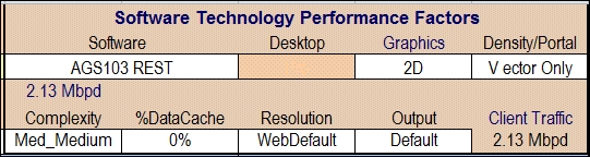
As shown here, you can specify the type of server, whether it's 2D or 3D, density, map complexity, percent cache, resolution, and output of services.
- A fast disk subsystem can make all the difference to performance. Work with your IT team or conduct some tests to determine optimal performance if you plan to develop the system from the ground up.
- If your app will publish a geoprocessing service, it's critical that it has the fastest clock speed you can purchase, because these kinds of operation are CPU intensive.
- For memory, Esri recommends 3 GB per core. A four-core server will need 12 GB of RAM.
- Network usage and capacity is critical to the relaying of data between your ArcGIS Server environment and the app. With the CPT, you can evaluate the service times of your app, based on current network use and capacity, and projected network use and capacity.
Geographic data is key to any mapping app so this section will list several techniques for making your app as fast as possible:
- Only add the layers that your app needs. It's tempting to add lots of layers because content is important. However, the more layers you add, the slower the app will be. Esri recommends adding layers in the 1s and 10s of layers.
- Cache your dynamic map services so that users see the data as images at the scale range where the user only needs to see the data.
- Add scale ranges to your layers so that they only show at the scale that they are needed.
- Evaluate the image format of image services, tiles services, and dynamic map services. The CPT allows you to determine the optimal format for these kinds of service.
- With the CPT, you can also test out different resolutions. If your app is going to be mostly used on a phone, choose a resolution of 256x256 or 400x300.
- If possible, generalize layers that have a large number of vertices. For example, if you need to display Chesapeake Bay and your layer has 3 million vertices, consider generalizing it to enough vertices so that it maintains its overall shape, while also removing vertices that aren't needed so that performance is maximized.
- Keep your data in the same spatial reference. Changing spatial references impacts performance, so if the data is all in the same spatial reference, there will be fewer on-the-fly re-projections.
- Optimize the performance of your enterprise geodatabase by following best practices for your DBMS. Consult your DBMS documentation for performance guidelines.
- Use definition queries on your layers when you set up the map to publish.
- Simplify the layer symbology. Avoid using complex symbols because they take longer to draw.
Please consult Esri's help for more details.
When it comes to ArcGIS Server, there are a few key tips to maximize performance:
- It's important that you have enough servers to handle incoming requests. With small setups, a single server will suffice, but with even a few dozen concurrent users, you may be required to have multiple ArcGIS Server installations.
- Increase the number of instances of your services so that more than one instance is handling an incoming request. For more details, navigate to http://www.wiki.gis.com/wiki/index.php/Server_Software_Performance#Service_instance.
Now that we've reviewed some things you can do on the server side, let's turn our attention to what we can do to make ArcGIS Runtime perform optimally. In order to discuss this subject, we're going to have to take a deeper dive into the rendering engine, and that means we will discuss Graphics Processing Unit (GPU), Central Processing Unit (CPU), and the decisions that one must make when deciding on how to render layers. Before we do that, however, we first need to understand a little about graphics programming APIs such as OpenGL and DirectX. ArcGIS Runtime SDK for .NET actually uses DirectX, but we're only going to discuss this at a high level, so these comments generally apply to OpenGL too.
When you add a layer to the map or scene using symbology individually or via a renderer, the layer is eventually rendered to the GPU. To understand how this works, we're going to talk very briefly about graphics programming. If you were to build your own mapping API, you would not only have to build your own data formats, tools, and so on, you'd also have to build a means to render this content to a GPU so that it renders it quickly.
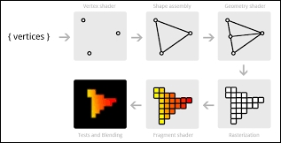
This process works by taking the original Esri geometries (with symbology applied) you created in geographic space and converting them into screen space as vertices, as shown here in the first image, in the upper-left corner of this screenshot:
Symbology applied
This presentation is the graphics pipeline. Note that these are vertices for graphics rendering to the GPU, which originally comes from the vertices we created with the Esri geometries. Once the vertices are in screen space, they are converted into triangles. It doesn't matter if the original geometry was an Esri point, line, or polygon, the symbol used to render them on the map is eventually converted into triangles. Here is an example of a polygon that has been converted into triangles:
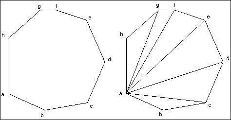
Conversion of polygon to triangles
Once it has been converted into a set of triangles, it is rasterized into pixels, and then the screen coordinates are converted into texture coordinates so that the original Esri symbol is displayed correctly on the GPU. Texturing is the process of converting graphic primitives, such as an Esri MapPoint class with a symbol, into a picture that can then be rendered on the GPU. Even if the symbol for the polygon is a simple blue color, this requires a texture that appears blue to be applied to the rasterized triangles (pixels) so that they appear correct to the human eye. Coloring is then applied by the GPU. Once that is complete, the final rasterized image is sent to the frame buffer, where it is rendered to the screen using an OpenGL or DirectX call.
Instead of texturizing the graphics, a more recent advancement has been made, called path rendering. In a basic sense, path rendering is the process of taking text or a graphic and drawing an outline around it, as shown in the preceding screenshot. Path rendering is much more precise-looking than textures, because textures are just pictures while paths are detailed outlines of the text or graphic. See here:

Texture and path
The F letter on the left is a texture (picture) while the F letter on the right is a path (outline). The outlined F letter is much more precise-looking. Path rendering has many advantages and has been created from the preceding graphics.
One other concept that you need to understand is that when you move though the graphics pipeline, this requires changes in state. Every step requires the graphics API to switch modes of operation. Moving from creating triangles to building a texture requires a change in what the GPU is doing. The goal of any graphics engine developer is to reduce the number of state changes that occur because they degrade performance.
Another goal of building a rendering API is to reduce the number of passes that the API has to make when producing an image. Take, for example, a tiled basemap. If you recall from earlier discussions, a tiled service or package is made up of pre-generated tiles that are just images. From the perspective of OpenGL or DirectX, these are just textures, which are added to the display one tile at a time. The primary goal of using OpenGL or DirectX is to reduce the number of times these tiles have to be passed over along with other layers to create a final image. Remember that a nontrivial map will contain several layers that contain basemaps, operational layers, and dynamic layers, which we discussed in Chapter 1, Introduction to ArcGIS Runtime. See here:
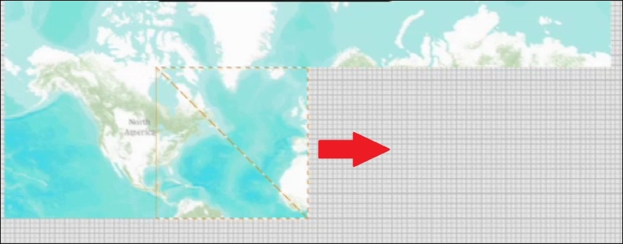
Generation of a basemap
As this basemap is generated, it requires that each tile is created as a texture and placed in its proper location. Each tile is added one at a time until the basemap is finished. Then, depending on how the other layers are configured, the remaining layers may be added while the basemap's tiles are added to the display, or they may not be added until another pass. It can take one or more passes to generate the final image that you actually see on the map. The Runtime Core gives you some control over how many passes it takes to generate an image.
For more information on how the graphics pipeline works with DirectX or OpenGL, see here:
https://msdn.microsoft.com/en-us/library/windows/desktop/ff476882(v=vs.85).aspx
Also see here:
ArcGIS Runtime comes with two ways of rendering your layers on the map or scene using the CPU or GPU:
- Static
- Dynamic
Static rendering is the process of rendering when the user finishes an operation, such as zooming in. Static rendering is primarily done through the CPU. Dynamic rendering is the process of always rendering to the GPU. Each of these modes has pros and cons to consider. Static rendering does not occur until there is a context change, that is, the completion of an operation such as a pan or zoom. When that occurs, the symbols appear to pop. In other words, they abruptly change from one size to another very quickly during a zoom in operation. The zoom operation is being handled by the CPU, but the rendering is the responsibility of the CPU or GPU, depending on the mode. Once the CPU has completed performing the zoom operation, the CPU takes over in static mode or the GPU takes over in dynamic mode. In other words, the rendering occurs on demand, that is, when a zoom operation completes. When in dynamic mode, this popping sensation does not occur, because the GPU is always rendering the Esri geometry (there is no context change).
Static mode is all about cartographic quality, and that is achieved with path rendering. The entire graphic is rendered as a path. The other big advantage of static mode is that it scales very well. The Runtime Core only regenerates textures when it needs to, when a change occurs in a part of the map. As a result, increasing or decreasing the number of features or graphics doesn't influence performance. The downside of static mode is that it can be memory intensive because it is CPU bound.
For dynamic mode, cartographic quality is sacrificed for improved performance. The reason for this is that textures are used instead of paths. These textures reside in a texture mosaic, which would look something like this:

A texture mosaic is simply a list of textures that come from your symbols in your layers. The texture mosaic always exists on the GPU, which means less work for the CPU, and that means less battery drain. Because it resides on the GPU, textures are very quickly accessed.
To set the rendering mode for your layers, you simply set the rendering mode with RenderingMode. Both feature layers and graphics layers support both static and dynamic mode. Tiled layers and map service layers only support static mode rendering, so the dynamic option isn't available for these layer types. When working in dynamic mode, the symbols are converted to graphic primitives, which are then converted into triangles and texturized, as we discussed in the previous section. These symbols are then rendered to the GPU. Static rendering converts the images to paths and renders them to the GPU.
When it comes to text and the labeling of layers, the Runtime Core uses path rendering instead of textures when in static mode. Starting with the 10.2.4 version of ArcGIS Runtime, the Runtime Core now uses texture fonts, which are stored in a texture mosaic on the GPU. Using this approach, the rendering engine can reuse letters on the texture mosaic.
Dynamic mode is best for rendering data during an animation or when navigating. This mode is excellent for tracking yourself using the built-in GPS because the system doesn't have to wait to render. That's because the graphics reside on the GPU at all times in a texture mosaic. As a result, the CPU isn't being used when panning, zooming, or rotating the map. This provides a smooth display experience, but it should be used sparingly when displaying a large number of features. For example, if you have 10,000 points on the map, 10,000 vertices have to be rendered to the GPU, which can result in display degradation. Furthermore, if the symbols are complex, this too can degrade performance. Along with this is that the cartographic quality isn't as good as it is with static mode. But the graphics are screen aligned so that if you rotate the map, the symbols and text stay aligned with how you set them, no matter the orientation of the map.
Static mode, on the other hand, is good for rendering lots of features on the map and achieving high cartographic quality (path rendering). But, because static mode relies more on the CPU, it consumes more of your battery and memory. Furthermore, if one graphic or feature changes, it will then require an update to an entire tile (tiled layer) or map image (dynamic map layer). Furthermore, if the map rotates, the graphics or text also rotate (they are not screen aligned).
So, which rendering mode should you use? Well, it depends on the balance between the number of graphics versus the GPU memory and power. Are you going to be offline? Is battery life a concern? Such similar factors need to be considered. It really comes down to the use case.
Static mode will create the same number of textures no matter the number of graphics, which consumes CPU cycles, which in turn burns battery power. Also, the number of layers and the order of the layers really play a role when in static mode. On the other hand, when in dynamic mode, graphics live in GPU memory all the time, so more graphics means more GPU processing power will be required, and that can result in a slower UI experience. This is especially the case if you have a large number of graphics and a slower GPU, such as on phones. The number of layers and their order is not as important as with static mode.
When in dynamic mode, the number and order of layers isn't that important because resources are shared between all layers on the GPU. It's important that the static layers are placed beside each other on the map, as this reduces the number of passes the rendering engine has to make. If you place a dynamic layer between two static layers, this requires a pass for all three layers. If you place the two static layers beside each other, only two passes are necessary. The reason for this is that the static mode layers don't share resources (textures). Even though the Runtime Core attempts to do some optimizations for you, it's important that you keep this in mind when adding layers to the map.
If a graphics or feature layer contains polygons, static mode is best for feature services if you don't know how many features there are, the kind of symbols used, or the geometry complexity. On the other hand, dynamic mode is good for sketching or interactive layers, real-time feeds, and point layers.
Now that we've covered some of the basics of how Runtime Core's display rendering engine works, let's consider how we can optimize graphics layers. Here are some recommendations:
- Use arrays or generics (
List<T>) when populating aGraphicsLayerclass. - Use a renderer whenever possible. The ArcGIS Runtime display engine will look at the graphics in a graphics layer and determine whether they have the same symbol. If they do, the engine will reuse the same texture once, no matter how many graphics are in the layer. If we add graphics individually, this requires converting the graphic to triangles, and then generating a texture. This is a state change. With hundreds or thousands of graphics being added, this also means hundreds or thousands of state changes, which is slower than using a renderer.
Using an ArcGIS Runtime renderer, on the other hand, only requires one state change if there is only one symbol used to make the renderer. As we will see, using a renderer will be much faster than adding graphics individually.
- You can add any kind of geometry to a
GraphicsLayerclass. However, if you add points and polygons to the same graphics layer, that means that the display engine has to switch states, which reduces performance. It switches states because it has to draw the points, generate textures, draw the polygons, generate the textures, and so on. - Avoid layer-level transparency because it requires two passes with the GPU, once for the original layer, and then again for the transparency. Symbol-level transparency will be more performant.
Let's now test some different ways of adding graphics to a map so that you can see some differences in performance, depending on how you add the graphics to the GraphicsLayer class. Look at the project called Chapter11c with the code that came with this book. First, let's add 50,000 graphics individually to a map, using a for loop:
// get the graphics layer
GraphicsLayer graphicsLayer = MyMapView.Map.Layers["graphicsLayer"]
    as GraphicsLayer;
this.random = new Random();

// create a stopwatch
Stopwatch stopWatch = new Stopwatch();
stopWatch.Start();

// create a bunch of graphics
for (int i = 0; i < 50000; i++)
{
    int latitude = random.Next(-90, 90);
    int longitude = random.Next(-180, 180);
    MapPoint mapPoint = new MapPoint(longitude, latitude);

    SimpleMarkerSymbol sms = new SimpleMarkerSymbol();
    sms = new Esri.ArcGISRuntime.Symbology.SimpleMarkerSymbol();
    sms.Color = System.Windows.Media.Colors.Red;
    sms.Style = Esri.ArcGISRuntime.Symbology.SimpleMarkerStyle.Circle;
    sms.Size = 2;
    Graphic graphic = new Graphic(mapPoint, sms);
    graphicsLayer.Graphics.Add(graphic);
}
// stop timing
stopWatch.Stop();
TimeSpan ts = stopWatch.Elapsed;

Console.WriteLine("Time elapsed: {0}", stopWatch.Elapsed);
Give this code a go and see how long it takes. Basically, it will add 50,000 points to the map in random locations using latitude/longitude.
Now that we've done this the slow way, let's try a couple of faster approaches. In the next example, let's add 50,000 graphics using a generic list that then has the graphics added to the GraphicsLayer.GraphicSource property:
// get the graphics layer
GraphicsLayer graphicsLayer = MyMapView.Map.Layers["graphicsLayer"]
        as GraphicsLayer;
this.random = new Random();

// create a stopwatch
Stopwatch stopWatch = new Stopwatch();
stopWatch.Start();

// create a enerable list
List<Graphic> graphics = new List<Graphic>(50001);
// create a bunch of graphics
for (int i = 0; i < 50000; i++)
{
    int latitude = random.Next(-90, 90);
    int longitude = random.Next(-180, 180);
    MapPoint mapPoint = new MapPoint(longitude, latitude);

    SimpleMarkerSymbol sms = new SimpleMarkerSymbol();
    sms = new Esri.ArcGISRuntime.Symbology.SimpleMarkerSymbol();
    sms.Color = System.Windows.Media.Colors.Red;
    sms.Style = Esri.ArcGISRuntime.Symbology.SimpleMarkerStyle.Circle;
    sms.Size = 2;
    Graphic graphic = new Graphic(mapPoint, sms);

    graphics.Add(graphic);
}
graphicsLayer.GraphicsSource = graphics;

// stop timing
stopWatch.Stop();
TimeSpan ts = stopWatch.Elapsed;

Console.WriteLine("Time elapsed: {0}", stopWatch.Elapsed);
Once you run this example code, you will see that it loads the graphics faster than the previous example, because the graphics are being assigned to the layer as a source directly.
One last example will illustrate adding the graphics using a simple renderer:
// get the graphics layer
GraphicsLayer graphicsLayer = MyMapView.Map.Layers["graphicsLayer"]
    as GraphicsLayer;
this.random = new Random();

// create a stopwatch
Stopwatch stopWatch = new Stopwatch();
stopWatch.Start();

SimpleMarkerSymbol sms = new SimpleMarkerSymbol();
sms = new Esri.ArcGISRuntime.Symbology.SimpleMarkerSymbol();
sms.Color = System.Windows.Media.Colors.Red;
sms.Style = Esri.ArcGISRuntime.Symbology.SimpleMarkerStyle.Circle;
sms.Size = 2;

SimpleRenderer simpleRenderer = new SimpleRenderer();
simpleRenderer.Symbol = sms;

// create a enerable list
List<Graphic> graphics = new List<Graphic>(50001);
// create a bunch of graphics
for (int i = 0; i < 50000; i++)
{
    int latitude = random.Next(-90, 90);
    int longitude = random.Next(-180, 180);
    MapPoint mapPoint = new MapPoint(longitude, latitude);
    Graphic graphic = new Graphic(mapPoint);
    graphics.Add(graphic);
}
graphicsLayer.Renderer = simpleRenderer;
graphicsLayer.GraphicsSource = graphics; ;

// stop timing
stopWatch.Stop();
TimeSpan ts = stopWatch.Elapsed;

Console.WriteLine("Time elapsed: {0}", stopWatch.Elapsed);
Using the laptop this book was written with, the times for each approach are summarized here:
|
Added graphics using |
Time (in seconds) |
|---|---|
|
Individually ( |
0.1866448 |
|
|
0.1078491 |
|
|
0.0429644 |
These are very fast times, because the laptop used has a high-end graphics card and processor. You may need to reduce the number of graphics when you try it on your PC or laptop. Regardless, from these simple changes we can easily see that when we change from adding the graphics individually to adding them with GraphicsSource, the time it takes to render them decreases by about 42 percent. When we go from GraphicsSource to using SimpleRenderer, the decrease in time is about 60 percent. When we go from adding graphics individually to a GraphicsLayer class to using SimpleRenderer, the time it takes to render the graphics decreases by about 77 percent. That's outstanding! You will of course get different results, depending on the symbology, number of graphics, and hardware (RAM, processors, and graphics card).
When it comes to working with layers, there are a few other tips you can use to improve performance:
- Limiting the number of fields in queries. Setting
Query.OutFields.Addto*is fine for a layer with a small number of fields, but using this approach with a large number of fields will degrade performance. - Excluding the geometry in your queries can greatly improve performance, especially with several features being returned or with complex geometries.
- Maintaining the same spatial references so that on-the-fly re-projections don't occur.
- When using the routing functionality, you can set the
OutputLinesproperty onOnlineRouteTask. Setting this option can reduce the response size of the data. - If your app is focused on a particular area of the world, make sure to set
InitialViewpointto that area. This can reduce the amount of data coming across the Internet. Note that it's not possible to do this with Windows Store and Phone via XAML; it can be done with code, however.