
Chapter 3
Flaws in Modern Financial Theory
As an aerospace engineer, my education kept me far removed from the world of finance. Over the past couple of decades my career dropped me solidly into the “world of finance.” The world of finance is my baked-up term that includes financial academia and, in general, retail (sell side) Wall Street. I honestly believe that the former is the marketing department of the latter.
In engineering we knew that to begin an analysis or delve into a research project, we had to begin with some basic assumptions about things. These assumptions were the starting blocks for the project; they launch the process. Many times, well into the project, it would be obvious that some of the assumptions were just wrong and had to be corrected or removed. The World of Finance over the past 60 years has produced a large number of white papers on financial theories, many of which begin with some basic assumptions. So far, so good!
- The markets are efficient.
- Investors are rational.
- Returns are random.
- Returns are normally distributed.
- Gaussian (bell-curve) statistics is appropriate for use in finance/investing.
- Alpha and beta are independent of correlation.
- Volatility is risk.
- Is a 60 percent equity/40 percent fixed income appropriate?
- Compare forward (guesses) Price Earnings (PE) with long-term trailing (reported) PE.
The remainder of this section covers the challenges I have to the above list. Personally, I think modern finance is almost a hoax, an area of investments that has proliferated into a gigantic sales pitch. Few challenge it, and even fewer fully understand it. I think I could write an entire book about the flaws of modern finance but will try to offer a number of examples of how shallow and truly ineffective some of the concepts are along with examples. Hopefully, I will be successful with some examples that it will at least bring concern on your part and further study into the subject.
I should state that it isn’t the problems of modern finance as much as how investment management cherry picks and misuses parts of it for marketing purposes.
What Modern Portfolio Theory Forgot or Ignored
Recall that the theory assumes that all investors obtain the same information at the same time. Also, that they react similarly and share the same investment goals. Here are some rhetorical questions to challenge those assumptions:
Do people trade/invest using different time horizons? There are now investors/traders who trade in extremely short intervals during the day. There are those who will never hold a position overnight. There are those who let the market determine their holding period. And there are those who buy and hold for very long periods of time.
Are there different views of risk among investors? The really sad part of this questions is that most investors do not fully understand risk and certainly do not know what their risk tolerance is, let alone how to apply it to an investment strategy.
Are there different views of where the same stock’s price will be one week, one month, or one year from now? This doesn’t need any explanation because if you read financial media or watch television you know there is an unlimited supply of opinions on this.
The Capital Asset Pricing Model (CAPM) assumes that investors agree on return, risk, and correlation characteristics of all assets and invest accordingly. They rarely do. Some of the problems with return, risk, and correlations are dealt with elsewhere in this book. The biggest is that most use very long-term averages of these to assess future valuations. They should use an average that adapts to an investor’s investing time horizon.
Modern Portfolio Theory and the Bell Curve
I’ll let Benoit Mandelbrot explain it from his book, The (Mis)Behavior of Markets (p. 13). The bell curve fits reality quite poorly. From 1916 to 2003, the daily movements of the Dow Industrials do not spread out on graph paper like a simple bell curve. The far edges flare too high. Theory suggests that over that time, there should be 58 days when the Industrials moved more than 3.4 percent; in fact, there are 1,001 such days. Theory predicts six days of swings beyond 4.5 percent; in fact, there were 366. And swings of more than 7 percent should come once every 300,000 years; in fact, there were 48 such days. Perhaps the assumptions were wrong. (B32)
Black Monday, October 19, 1987
“The Dow Jones Industrials fell 29.2 percent. The probability of that happening, based on the standard reckoning of financial theorists, was one in 10 to the 50th power; odds so small that they have no meaning. It is a number outside the scale of nature. You could span the powers of ten from the smallest subatomic particle to the breadth of the measurable universe—and still never meet such a number,” The (Mis)Behavior of Markets, Benoit Mandelbrot (B32). Without knowing how he calculated the returns (daily, weekly, etc.) and the amount of data used in the calculation, it is impossible to re-create his numbers. He stated that on Black Monday the Dow Industrials fell 29.2 percent. Here are the numbers: October 16, 1987, close price was 2,246.74, October 19, 1987, close price was 1,738.74, which is a decline of 22.61 percent. If one used the low of October 19, 1987 (1,677.55), the decline would be −25.33 percent. The message is, however, the same; it was a huge decline and one that statistically should never happen. (B32)
Figure 3.1 shows the huge difference between the distribution of returns from the Gaussian “normal distribution” and the actual distribution of empirical data. This is the daily return of the Dow Industrials from 1885 with the vertical axis being relative probability and the horizontal axis being percent return. The taller peak is the Gaussian normal distribution and the other is the actual returns. You can see the small dot at the far left representing the −22.61 percent day known as Black Monday, October 19, 1987.

FIGURE 3.1 Normal Distribution Versus Actual Distribution from 2/17/1885 to 12/31/2012
Tails Wagging the Dog
If an asset bubble is defined as 2 standard deviations (σ, sigma) about its mean, then . . . statistically it won’t happen but once every 43 years (four sigma total). Statistics dictate that only once every 1,600 years should such events be followed by a reverse move downward of 2 standard deviations. Sadly, these events happen often. Hence, once again, Gaussian statistics are not appropriate for market data. (B32)
October 2008 had some rare events. Table 3.1 shows 11 days during October 2008 ordered by absolute daily return.
| 2008 | Return |
|---|---|
| October 13 | 11.1% |
| October 28 | 10.9% |
| October 15 | −7.9% |
| October 9 | −7.3% |
| October 22 | −5.7% |
| October 7 | −5.1% |
| October 16 | 4.7% |
| October 20 | 4.7% |
| October 24 | −3.6% |
| October 6 | −3.6% |
| October 2 | −3.2% |
TABLE 3.1 October 2008
The top three days based upon absolute daily returns are 11.1 percent, 10.9 percent, and −7.9 percent. The mathematical odds of three days with greater than 7.9 percent moves is: 1 in 10,000,000,000,000,000,000,000 (that’s 10 plus 21 zeros). The rise of the term fat tails recently is because the world of finance uses the wrong statistical analysis for the market. If the correct analysis were used, the term fat tails would not be used, it would have been addressed. This example reminds me of the e-Trade baby exclaiming that the odds are the same as if being eaten by a polar bear and a regular bear in the same day. While I’m critical of the statistics used in modern finance, I think I’m more concerned about their widely held belief as being valid. If you know something has problems, you can adjust accordingly. If you do not realize there are problems, you are in trouble.
My friend Ted Wong (TTSWong Advisory) has this to say about modern finance: “After Markowitz introduced Modern Portfolio Theory (MPT) in the 1950s, which was based on the Gaussian hypothesis, most theoreticians had since moved away from Gaussian statistics. Only the naive research analysts in the financial wire-houses and mutual fund institutions still use normal distributions in their papers. In fact, Benoit Mandelbrot cited in your book was the first to point out in the mid-1960s that the bell curve could not explain many fat tails observed in nature and in the financial markets. Fama and French pointed out that Gaussian statistics was only a special case in the family of Paretian distributions. The latter could account for all forms of fat tails by adjusting the leptokurtosis coefficient.” [Author’s note: Paretian refers to stable distributions, which should be used in modern finance but are rarely used because the mathematics is more complex, anyway that is my opinion. James Weatherall, in The Physics of Wall Street, provides a unique history of how Mandelbrot challenged modern finance and made headway, but ultimately did not change anything. (B59)]
“To me, the underlying problem with modern finance is not that Gaussian distributions don’t fit the fat tails well. By adjusting the leptokurtosis coefficient, the quasi bell curve can now be bent by the theoreticians to whatever shapes and forms to fit the empirical data. The real issue in modern finance is the “blind” faith in the random walk hypothesis. Both the MPT and the Paretian practitioners assume that market prices behave in a random fashion. The random walk doctrine assumes that price changes are independent variables; that is, today’s price change has no relationship with yesterday’s or tomorrow’s price change. They have hundreds of “proofs” to back up that claim and as a result, financial academia laughs at technical and even fundamental analysts in their efforts to predict future market prices.
“What the random walkers miss is the fact that most technical and quantitative analyses are not intended for predicting daily price changes, which I agree are more or less random. We believe that market prices are not random over a longer period of time. The distributions of totally random price events should have the mean near 0 percent and surrounded by a symmetrical distribution on either side just like the bell curve or the Paretian curve (with fat tails on both sides). If the mean return is located off center and the distributions are asymmetrical around the mean, then one can surely challenge the notion of randomness. Well, look at your Figure 2.1, it’s a clear demonstration that over a one-year period, the mean percent return is off center to the right, and the distributions are asymmetrical around the mean. Hence the historical annual return histogram proves that the market is not random. The longer the holding period, the less random (thus more predictable) the market is! Random walks are only random when one walks a short time distance. One can rightfully say that day traders are true random walkers and that technical analysis may not be as useful to them.”
Standard Deviation (Sigma) and Its Shortcomings
Warning: This section is for nerds only!
Definition: A light year is a distance not a time. It is the distance that light will travel in one year.
Table 3.2 has some numbers that are beyond human capacity to imagine. They are beyond our ability to comprehend. In my normal overkill fashion my goal here is to put these giant numbers into a believable perspective so you will believe that something is wrong with the statistics of modern finance. Black Monday, October 19, 1987, was a decline of 22.61 percent, which was approximately 22 sigma. Twenty-two sigma as shown in Table 3.2, based on Gaussian statistics, should only occur once in every 9.5 × 10103 years. That needs to be put into perspective. The speed of light is approximately 186,282 miles per second, so the speed of light in miles per hours is 186,282 × 60 × 60 = 670,615,200 miles per hour. Further expansion shows that the speed of light per day is 670,615,200 × 24 = 16,094,764,800 miles per day and so the speed of light per year is 16,094,764,800 × 365.25 = 5,878,612,843,200 miles per year. In scientific notation this is expressed as 5.878 × 10¹². Note that this number is similar to the value for eight sigma (see Table 3.2). To create an impression of sigma that is greater than eight would require the use of terms that deal with the universe, yet I’m going to give it a shot.

TABLE 3.2 Probability of Events Occurring
Here is a list of galactic-like measurements to help put large sigma events into perspective. There are many wonderful websites on astronomy and such. I checked a number of them and found a general agreement with the numbers used in these examples. Keep in mind that the numbers were generated with a scientific approach, not just a guess, but still could be in considerable error. Most of the information can be found on www.universetoday.com.
How many stars are there in the Milky Way galaxy? I found that from a number of different sources this number was fairly consistent and is about 2,500 that are visible to the naked eye on Earth at any one time and 5,800 to 8,000 total visible stars. Now here is the guess of astronomers for the total number of stars in the Milky Way: 200 billion to 400 billion (4 × 10¹²). Now the Milky Way galaxy is a spiral galaxy that is approximately 100,000 light years across, so you can see that we truly do not know a precise answer other than there are billions of stars in the Milky Way galaxy.
How many galaxies are in the universe? Because we can only see a fraction of the universe, this is impossible to know, but most astronomers have said that there are 100 billion to 200 billion galaxies in the universe. Their recent supercomputer put the number at more than 500 billion, in other words there is an entire galaxy for every star in the Milky Way.
The obvious next question then is how many stars in the universe? Since the determination for the number of galaxies in the universe and the number of stars in each galaxy is clearly a wide-ranging estimate, I’ll just use something near the middle of the estimates (aren’t you glad I did not use average?). Then, 400 billion galaxies and 400 billion stars in each galaxy equate to 160 trillion stars in the universe. In scientific notation that is (4 × 1012) × (4 × 1012) = 1.6 × 1025. That’s a lot of stars, but keep in mind the purpose of this cosmic exercise is to get a perspective on high sigma events. Looking at Table 3.2 you can see that this is close to about an 11 sigma event.
How many atoms in the universe? Let’s use the conservative of the estimates just to keep it exciting. If there are 300 billion galaxies in the universe and the number of stars in a galaxy can be 400 billion, then the total number of stars in the universe would be about 1.2 × 10²³. Always refer to the sigma table to see where these numbers stand relative to large sigma events to keep them in perspective. UniverseToday estimates that on average (there’s that concept again) each star can weigh 1035 grams. Therefore, the total mass of the universe would be about 1058 grams (Note: Multiplication of exponents is easy, just add them: 23 + 35 = 58). Because a gram of matter is known to have about 1024 protons (same as the number of hydrogen atoms), then the total number of atoms in the universe is about 1082. From Table 3.2 you can extrapolate and see that it is about the same as a 19 sigma event occurring—and Black Monday, October 19, 1987, was a 22 sigma event.
What is the age of the universe? NASA’s Wilkinson Microwave Anisotropy Probe has pegged the answer to 13.73 billion years, with a margin of error down to only 120 million years (1.2 × 10⁸).
What is the age of the Earth? Plate tectonics has caused rocks to be recycled so it makes it difficult to actually determine the Earth’s age. They have found rocks in Michigan and Minnesota that are about 3.6 billion years old (3.6 × 10⁹). Western Australia has yielded the oldest rocks thus far at 4.3 billion years. Moon rocks and meteorites have yielded about 4.54 billion years on average, which is also science’s determination for the age of the solar system.
What about humans? Currently (seems they are always finding something older) the first homo habilis evolved about 2.3 million years ago—these were the folks that used stone tools and probably not too different than a chimp. According to Recent African Ancestry theory, modern humans evolved in Africa and migrated out of the continent about 50,000 to 100,000 years ago. The forerunner for anatomically modern humans evolved between 400,000 and 250,000 years ago. Finally, many anthropologists agree that the transition to behavioral modernity (culture, language, etc.) happened about 50,000 years ago. We humans are certainly a tiny fraction compared to the universe, and in particular, large sigma events.
Okay, I have thoroughly beat this “perspective” idea to death but hope you found the galactic information entertaining. Basically, and practically, any sigma greater than 4 is usually addressed as infinity. Moreover, in the case of the stock market, that means these events should never happen, yet they do. And way too often! Table 3.2 shows various sigma, the percent of population, the probability of exceeding that sigma, and a calendar based interpretation. I have noticed that Microsoft Excel and Wolfram Alpha produce slightly different values. I think even with the best of intentions when dealing with extremely large or small numbers, one simple rounding error or inappropriate rounding can lead to differences, however, it did not affect the message here.
Improper Process
When diving into this project on standard deviation and large market moves, I realized that all too often, analysts who are showing similar information are making an egregious error in the calculation. If you wanted to know the standard deviation (sigma) for October 19, 1987 (Black Monday), then you cannot use any data later than or including that day to determine it. I see many times that one will use the calculation of standard deviation on a daily basis up to the day of the analysis, which often includes many years of data that did not exist at the time of the event being analyzed. Table 3.3 shows the 10 largest percentage days in the Dow Industrials since 1885. The Correct Sigma column shows the calculation for past data up to the day before the event, while the Spot Sigma column shows the calculation for the day in question using all the data available up to 12/31/2012, which I don’t believe is valid. However, you will notice that there is not a huge difference in the two columns. That is, until you look at the difference and put it into a perspective that the human brain can deal with.

TABLE 3.3 Different Results for Sigma If Not Using Correct Data Periods
High Sigma Days We All Remember
In an attempt to portray certain days in the past that we have heard much about, the calculation of sigma expected and observed prior to those days is presented here for events from one sigma up to and including eight sigma. You will notice that at the high sigma data in the tables some of the data was entirely too large or too small to include. Also, the days we are discussing in the section were all much greater than eight sigma days. This analysis is to once again show how often we experience moves in the market that our completely beyond the boundaries of modern finance. Here are the explanations of the headers in the following three tables, October 28 to 29, 1929, October 19, 1987, and all the data up to 12/31/2012.
- Sigma—Standard deviation
- AM – xSD—Percent move representing the average mean (AM) less an “x” sigma move.
- Expected—The number of events expected using statistics.
- Observed—The actual number of events.
- Ratio—The ratio of expected to observed events.
- AM + xSD—Percent move representing the average mean (AM) plus an “x” sigma move.
- Expected—The number of events expected using statistics.
- Observed—The actual number of events.
- Ratio—The ratio of expected to observed events.
- Total Expected—The total of events expected above and below the mean.
- Total Observed—The total of actual events above and below the mean.
- Ratio—The ratio of the Total Expected and Total Observed events.
- AM – xSD—Percent move representing the average mean (AM) less an “x” sigma move.
Black Monday, October 28 and Black Tuesday, October 29, 1929
Table 3.4 shows the limits for one to eight standard deviations around the arithmetic mean (AM) return for the period from 2/17/1985 until the day before Black Monday, October 28, 1929. There were actually two significant declines during this period. On Monday, October 28, 1929, the Dow Industrials declined 12.82 percent, followed by Tuesday, October 29, 1929, with a decline of 11.73 percent. The total decline from the high price on Monday to the low price on Tuesday was more than 28 percent.
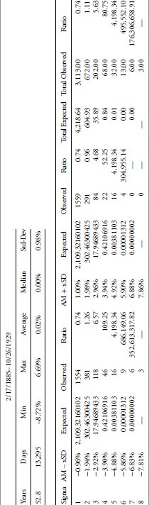
TABLE 3.4 Black Monday–Tuesday, October 28–29, 1929
To access an online version of this table, please visit www.wiley.com/go/morrisinvestingebook.
Black Monday, October 19, 1987
Table 3.5 shows the limits for one to eight sigma around the arithmetic mean (AM) return for the period from 2/17/1985 until the day before Black Monday, October 19, 1987. Black Monday’s decline was 22.61 percent, which is less than the two-day decline in October 1929. However, it was twice as large as Black Tuesday, October 29, 1929, which is the day recognized by most historians as the day of the crash.

TABLE 3.5 Black Monday, October 19, 1987
To access an online version of this table, please visit www.wiley.com/go/morrisinvestingebook.
1885–2012
Table 3.6 shows the limits for one to eight sigma around the arithmetic mean (AM) return for the period from 2/17/1885 until 12/31/2012.
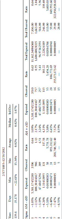
TABLE 3.6 Full History (1885–2012) of Daily Dow Industrials
To access an online version of this table, please visit www.wiley.com/go/morrisinvestingebook.
Rolling Returns and Gaussian Statistics
This section attempts to show that high sigma is a much more frequent event than modern finance thinks it is. A number of examples using the Dow Industrials back to 1885 on a daily basis are shown. Each begins with determining a look-back period to determine the average daily return and the standard deviation, and then a look-forward period is determined to see if the look-back data continues into the look-forward data. Figure 3.2 is an attempt to help visualize this process. A look-back period is determined (in-sample data) and a look-forward period is also determined (out-of-sample data). The look-back period is used to determine the average daily return and the standard deviation of returns. From that data a range of three sigma about the mean is determined. Then in the look-forward data, the number of daily returns outside the +/– three sigma band are tallied with the total being displaying as a plot; any point on the plot represents the data used in the look-back and the look-forward periods.
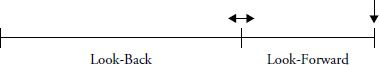
FIGURE 3.2 Visual for Look-Back, Look-Forward, and Data Point
In Figure 3.3 a look-back period of 1,260 days (five years) is used to calculate an average daily return and the standard deviation of returns. On 10/24/2002 (circle on Figure 3.3) the average return over the past 1,260 days was 0.07 percent, and the standard deviation over the same period was 0.71 percent. Therefore a three sigma move up was up to 2.21 percent, and a three sigma move down was −2.06 percent. The look-forward period, also 1,260 days, is counting the number of days in which the returns were outside of the look-back range. There were 49 days with returns greater than 2.21 percent and 69 days with returns less than −2.06 percent, for a total number of days with returns outside the +/–3 sigma range (based on the previous five years) equal to 118. Table 3.7 puts this into another format.
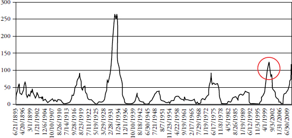
FIGURE 3.3 Five-Year Look-Back and Five-Year Look-Forward Days Outside +/− 3 Sigma

TABLE 3.7 Table Showing Data in Figure 3.3
For a +/– 3 sigma event the expected number of observations should be 1.7, whereas there were 118, which is 59 times more than expected (events must be in whole numbers so used 2 for the expected number). Figure 3.3 shows the 1,260-day rolling total number of days outside the +/– 3 sigma range. As of 12/31/2007 (five years ago) the total is 116, with an expectation of only 1.7. This is more than 58 times more returns outside the +/– 3 sigma band than expected. Of those 116 days outside the three sigma band, 54 were above 2.45 percent and 62 were below −2.37 percent.
Reducing the look-forward period to one year (252) days while maintaining the five year look-back period yields the chart in Figure 3.4 of rolling number of days outside a +/– 3 sigma (standard deviation) event. Remember that the determination of +/– 3 sigma is determined by the previous five years of data at any point on the chart. For a one-year look-forward there is only an expectation of 0.34 events (days) outside the sigma band.
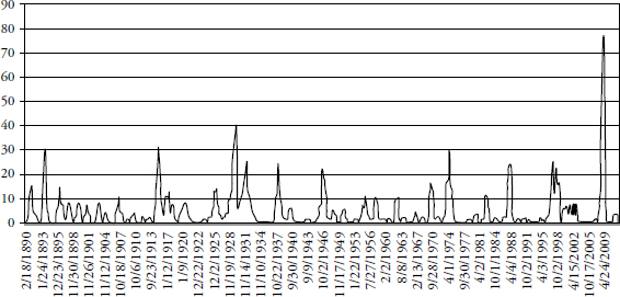
FIGURE 3.4 Five-Year Look-Back and One-Year Look-Forward Days Outside +/− 3 Sigma
Taking this concept to another view, Figure 3.5 shows the rolling number of days outside the +/– 3 sigma band for a look-forward of one year and a look-back of 10 years (2,520 days).
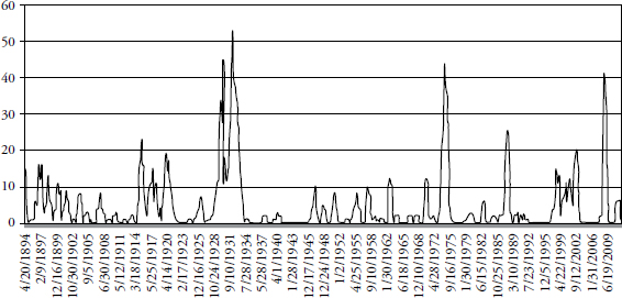
FIGURE 3.5 Ten-Year Look-Back and One-Year Look-Forward Days Outside +/– 3 Sigma
Keeping the look-forward period to one year and expanding the look-back period to 20 years (5,020 days) is shown in Figure 3.6. This chart is quite similar to the previous one with only a 10-year look-back. Extrapolating the past into the future always has its surprises. Keeping the look-forward period the same (one year) and increasing the look-back period does not significantly affect the rolling returns outside the sigma range.
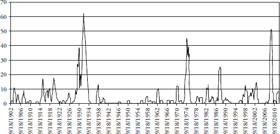
FIGURE 3.6 Twenty-Year Look-Back and One-Year Look-Forward Days Outside +/– 3 Sigma
Finally, in Figure 3.7, taking a 50-year look-back period (12,600 days), as expected the number of times the following year had exceeded the +/– 3 sigma envelope was similar.
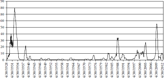
FIGURE 3.7 Fifty-Year Look-Back and One-Year Look-Forward Days Outside +/– 3 Sigma
Bottom line: Gaussian (bell-curve) statistics are not appropriate for market analysis, yet modern finance is totally wrapped up in using standard deviation as volatility and then saying that is risk. There are actually two big problems: one is the use of standard deviation to represent risk, and two is that past standard deviation has very little to do with future standard deviation. The first problem does not account for the fact that standard deviation (sigma) is also measuring both upside moves and downside moves with no attempt to separate the two. Clearly, upside volatility is good for long-only strategies. The second problem was adequately covered in this section showing how inadequate standard deviation is from the past in predicting how it would be in the future.
Risk and Uncertainty
Is volatility risk? (Here we go again.)
In the sterile laboratory of modern finance, risk is defined by volatility as measured by standard deviation; however . . .
- It assumes the range of outcomes is a normal distribution (bell curve).
- Rarely do the markets yield to normal.
When an investor opens his or her brokerage statement. . . .
It shows the following portfolio data for the last year:
- Standard Deviation =.65
- Loss for the Year = −35 percent
Which one do you think will catch their attention? I seriously doubt any investor is going to call his or her advisor and complain about a standard deviation of .65. However, the −35 percent loss will get their attention. Even investors who have no knowledge of finance or investments know what risk is—it is the loss of capital.
Risk is not volatility; it is drawdown (loss of capital). However, in the short term, volatility is a good proxy for risk, but over the longer term, drawdown is a much better measure of risk. Volatility does contribute to risk but it also contributes to market gains.
Risk and uncertainty are not the same thing.
Risk can be measured.
Uncertainty cannot be measured.
A jar contains five red balls and five blue balls. In the old days we called it an urn instead of a jar.
Blindly pick out a ball.
What are the odds of picking a red ball? There are five red balls and the total number of balls is 10. Therefore the odds of picking a red ball are 5/10 =.5 or 50 percent.
That is Risk! It can be calculated.
Suppose you were not told the number of red or blue balls in the jar.
What are the odds of picking a red ball?
That is Uncertainty!
Figure 3.8 is an attempt to visualize how modern finance is focused on risk, but have you ever wondered or thought about which element of risk they deal with? Actually they do a great job of analyzing risk; risk is at the heart of all the theories of Modern Portfolio Theory (Capital Asset Pricing Model, Efficient Market Hypothesis, Random Walk, Option Pricing Theory, etc.). The risk that they attempt to determine is known as nonsystematic risk, or you may have heard it as diversifiable risk. Diversification is a free lunch and should never be ignored. The world of finance is focused on diversifiable or nonsystematic risk. However, there is a much larger piece of the risk pie, and that is called systematic risk. Once you have adequately diversified, then it seems that you are only dealing with systematic risk. Systematic risk is what technical analysis attempts to deal with. It is also known as drawdown, loss of capital, and in certain situations as a bear market.

FIGURE 3.8 Nonsystematic and Systematic Risk
Back to the Original Question: Is Volatility Risk?
Two simple price movements are shown in Figure 3.9; which represents more risk, example A or example B?

FIGURE 3.9 Volatility versus Risk
Modern finance would have you believe that A is riskier because of its volatility. However, you can notice from this overly simple example that the price ended up exactly where it began, therefore you did not make money or lose money. B, based on the concept of volatility as risk, has no risk according to theory, however, you lost money in the process. I think it is obvious which is risk and which is only theory.
Is Linear Analysis Good Enough?
Figure 3.10 is known as a Cartesian coordinate system, sometimes referred to as a scatter diagram, used often to compare two issues and derive relationships between them. The returns of one are plotted on the X axis (abscissa/horizontal) and the returns of the other are plotted using the Y axis (ordinate/vertical). Those small diamonds are the data points. A concept known as regression is then applied by calculating a least squares fit of the data points. This is the straight line that you see below. Then a little high school geometry is used on the equation for a straight line, which is y = mx + b, where m is the slope of the line, and b is the where the line crosses the Y axis or y–intercept. So once you have the linearly fitted line, you can measure the slope and y–intercept and this will give you the beta (slope) and alpha (y-intercept).
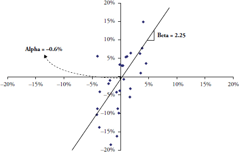
FIGURE 3.10 Source of Alpha and Beta from Linear Analysis
The following statistical elements can all be derived from simple linear analysis.
- Raw Beta
- Alpha
- R2 (Coefficient of Determination)
- R (Correlation)
- Standard Deviation of Error
- Standard Error of Alpha
- Standard Error of Beta
- t-Test
- Significance
- Last T-Value
- Last P-Value
Linear Regression Must Have Correlation
Figure 3.11 is a scatter plot of a fictional fund ABC (Y axis) plotted against the S&P 500 (X axis). The least squared regression line is plotted and the equation is shown as:
Y = 0.5997x + 0.0005, which means the slope is .5997 and the y-intercept is 0.0005.
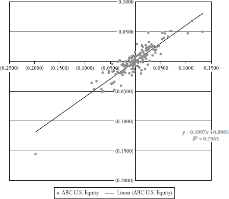
FIGURE 3.11 ABC U.S. Equity
A slope of 1.0 would mean that the Beta of the fund compared to the index was the same and the line on the plot would be a quadrant bisector (if the plot were a square, the line would be moving up and to the right at 45 degrees). So, a slope of 0.5997 means the fund has a lower beta than the index. The y-intercept is a positive number, although barely, but that means the fund outperformed the index.
R2 is the Coefficient of Determination, also known as the goodness of fit. Now I understand that dealing with positive numbers has some advantages, but in most cases R2 is also reducing the amount of information. Let me explain. We know that R is correlation, the statistical measure that shows the relationship between two datasets and how closely they are aligned. That is not the textbook answer for correlation, but will suffice for now. Correlation ranges from +1 (totally correlated) to −1 (inversely correlated), with 0 being noncorrelated. Nice information to know; is the fund correlated to the market, inversely correlated to the market, or not correlated at all. Squaring correlation will give you an always positive number (remember least squares?) but why remove the information about the level of correlation? R2 will not tell you if it is correlated or inversely correlated. Actually, I think it is the social science’s fear of negative numbers. However, in fairness, R2 will show the percent dependency of one variable over the other—in theory.
The R2 in Figure 3.11 is 0.7965, which means there is a fair degree of correlation, we just don’t know if it is positive correlation or inverse correlation. To get correlation, merely take the square root of 0.7965 to get R = 0.8924684 (yes, an attempt at humor), which means R could also be −0.8924684. Anyway, hopefully you get my point.
Finally, notice how the data points are all clustered fairly closely to the least squares line, which visually shows you that this fund is fairly well correlated to the index.
Figure 3.12 shows fund XYZ plotted against an index. Notice that the linear least squared fit equation (y = 0.5997x + 0.0005 is exactly the same as the previous example. However the value of R2 is 0.2051, which is considerably different than the previous example. Visually, you can see that the data points are more scattered than in the previous example so just based on the visual observation you know this fund is not nearly as correlated as the previous fund ABC. Yet, we find that the least squares regression line is oriented exactly the same so the values of alpha and beta are the same for this fund (XYZ) as they were for fund (ABC) above.
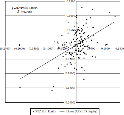
FIGURE 3.12 XYZ U.S. Equity
So what’s the difference, you are hopefully asking? The difference is that one fund is not nearly as correlated as the other. We know that they are both positively correlated from visual examination, but unless the value of R (correlation) is shown, we don’t know any more about the correlation. This is one of the horrible shortcomings of this type of analysis. Here is the message: If it isn’t correlated, then the values derived for alpha and beta are absolutely meaningless. Yet I see publications ranking funds and showing R2, alpha, and beta but never a mention of R. Shame on them!
The scatter plot in Figure 3.13 shows both funds plotted with the index. You can clearly see that fund XYZ (triangles) is not nearly as correlated as fund ABC (circles). Yet, the linear statistics of modern finance does not delineate a difference between the two. My only comment to them is: Stay out of aviation.
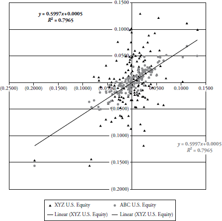
FIGURE 3.13 ABC and XYZ U.S. Equity
The 60/40 Myth Exposed
It is almost impossible to see any performance comparisons that not only show a benchmark, but also show a mix of 60 percent equity and 40 percent fixed income, known as 60/40 in the fund industry. The efficient frontier is one of those terms that came from a theory developed decades ago on risk management. Modern finance looks at a plot of returns versus risk, and, of course, by risk, it means standard deviation. This is the first mistake made with this concept. Then it plots a variety of different asset classes on the same plot and derive the efficient frontier, which shows you the level of risk you take for the asset classes you want to invest in. Figure 3.14 shows that efficient frontier curve from 1960 to 2010 (an intermediate bond component was used). Next, if you draw a line that is tangent with the curve and have it cross the vertical return axis at the level for assumed risk free, then the point of tangential is the proper mix of equity and bonds. I did not attempt to do this here as the determination of the risk free rate to use over a 50-year period presents too much subjectivity. From 1960 to present, that mix of stocks and bonds is about 60/40.

FIGURE 3.14 Efficient Frontier (1960–2010)
The ubiquitous 60/40 ratio of stocks to bonds, which shows up in most performance comparisons, gleans the message that for over 50 years of data nothing has changed? Does anyone actually believe that? Figure 3.15 is a chart showing the efficient frontier for each individual decade in the 1960 to 2010 period. Clearly each decade has its own efficient frontier and its proper mix of equity and bonds. Yet, the world of finance still sticks to the often wrong mix of 60/40. It may very well be a good mix of assets, but the data says it is dynamic and should be reviewed on a periodic basis. Notice that the decades of 1970 and 2000 showed similar downward curves meaning that stocks were not nearly as good as bonds. Conversely the decades of 1980 and 1990 were the opposite.

FIGURE 3.15 Efficient Frontier—Each Decade from 1960 to 2010
In an interview with Jason Zweig on October 15, 2004, Peter Bernstein said that a rigid allocation policy like 60/40 is another way of passing the buck and avoiding decisions. Did you want to be 40 percent invested in bonds during the 1970s when interest rates soared? Did you want to only be invested 60 percent in equities in the period from 1982 to 2000, which was the greatest bull market in history? Of course not! Markets are dynamic and so should investment strategies. Finally, some analysis will show that a 60/40 portfolio is highly correlated to an all equity portfolio.
Discounted Cash Flow Model
When studying modern finance, and after years of hearing about the discounted cash flow (DCF) model, I have this to say about the discounted cash flow model. First of all, you must decide on six values about the future. They are shown below. If you have read this book this far, you probably know what is coming next.
- Discount Rate
- Cost of Equity, in valuing equity
- Cost of Capital, in valuing the firm
- Cash Flows
- Cash Flows to Equity
- Cash Flows to Firm
- Growth (to get future cash flows)
- Growth in Equity Earnings
- Growth in Firm Earnings (Operating Income)
The inputs (above) to the DCF process must all be correct or the model fails completely. The odds of successfully coming up with correct (guesses) inputs are extremely low, yet this is used in modern finance routinely. This reminds me of the Kenneth Arrow story on forecasting in Chapter 5. When asked about the discounted cash flow model, I liken it to the Hubble Telescope; move it an inch and all of a sudden you are looking at a different galaxy.
The goal of this chapter at the very minimum is to cause you to challenge what modern finance has provided. I apologize for beating some concepts with a stick but sometimes multiple approaches to show something are better in the hope that one will remain with the reader. There was enough math to scare the average person, the next chapter focuses on the wide use of the term average. The goal is to show that using long-term averages can be totally inappropriate for most investors.