CHAPTER 15

OTHER TOPICS IN THE USE OF REGRESSION ANALYSIS

This chapter surveys a variety of topics that arise in the use of regression analysis. In several cases only a brief glimpse of the subject is given along with references to more complete presentations.

15.1 ROBUST REGRESSION

15.1.1 Need for Robust Regression

When the observations y in the linear regression model y = Xβ + ε are normally distributed, the method of least squares is a good parameter estimation procedure in the sense that it produces an estimator of the parameter vector β that has good statistical properties. However, there are many situations where we have evidence that the distribution of the response variable is (considerably) nonnormal and/or there are outliers that affect the regression model. A case of considerable practical interest is one in which the observations follow a distribution that has longer or heavier tails than the normal. These heavy-tailed distributions tend to generate outliers, and these outliers may have a strong influence on the method of least squares in the sense that they “pull” the regression equation too much in their direction.

For example, consider the 10 observations shown in Figure 15.1 The point labeled A in this figure is just at the right end of the x space, but it has a response value that is near the average of the other 9 responses. If all the observations are considered, the resulting regression model is ŷ = 2.12 + 0.971x, and R² = 0.526. However, if we fit the linear regression model to all observations other than observation A, we obtain ŷ = 0.715 + 1.45x, for which R² = 0.894. Both lines are shown in Figure 15.1. Clearly, point A has had a dramatic effect on the regression model and the resulting value of R².

Figure 15.1 A scatter diagram of a sample containing an influential observation.

One way to deal with this situation is to discard observation A. This will produce a line that passes nicely through the rest of the data and one that is more pleasing from a statistical standpoint. However, we are now discarding observations simply because it is expedient from a statistical modeling viewpoint, and generally, this is not a good practice. Data can sometimes be discarded (or modified) on the basis of subject-matter knowledge, but when we do this purely on a statistical basis, we are usually asking for trouble. We also note that in more complicated situations, involving more regressors and a larger sample, even detecting that the regression model has been distorted by observations such as A can be difficult.

A robust regression procedure is one that dampens the effect of observations that would be highly influential if least squares were used. That is, a robust procedure tends to leave the residuals associated with outliers large, thereby making the identification of influential points much easier. In addition to insensitivity to outliers, a robust estimation procedure should produce essentially the same results as least squares when the underlying distribution is normal and there are no outliers. Another desirable goal for robust regression is that the estimation procedures and reference procedures should be relatively easy to perform.

The motivation for much of the work in robust regression was the Princeton robustness study (see Andrews et al. [1972]). Subsequently, there have been several types of robust estimators proposed. Some important basic references include Andrews [1974], Carroll and Ruppert [1988], Hogg [1974, 1979a,b], Huber [1972, 1973, 1981], Krasker and Welsch [1982], Rousseeuw [1984, 1998], and Rousseeuw and Leroy [1987].

To motivate some of the following discussion and to further demonstrate why it may be desirable to use an alternative to least squares when the observations are nonnormal, consider the simple linear regression model

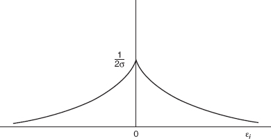
Figure 15.2 The double-exponential distribution.

where the errors are independent random variables that follow the double exponential distribution

The double-exponential distribution is shown in Figure 15.2. The distribution is more “peaked” in the middle than the normal and tails off to zero as goes to infinity. However, since the density function goes to zero as goes to zero and the normal density function goes to zero as goes to zero, we see that the double-exponential distribution has heavier tails than the normal.

We will use the method of maximum likelihood to estimate β₀ and β₁. The likelihood function is

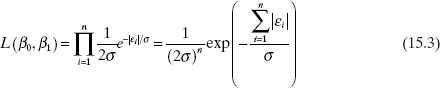
Therefore, maximizing the likelihood function would involve minimizing the sum of the absolute errors. Recall that the method of maximum likelihood applied to the regression model with normal errors leads to the least-squares criterion. Thus, the assumption of an error distribution with heavier tails than the normal implies that the method of least squares is no longer an optimal estimation technique. Note that the absolute error criterion would weight outliers far less severely than would least squares. Minimizing the sum of the absolute errors is often called the L₁-norm regression problem (least squares is the L₂-norm regression problem). This criterion was first suggested by F. Y. Edgeworth in 1887, who argued that least squares was overly influenced by large outliers. One way to solve the problem is through a linear programming approach. For more details on L₁-norm regression, see Sielken and Hartley [1973], Book et al. [1980], Gentle, Kennedy, and Sposito [1977], Bloomfield and Steiger [1983], and Dodge [1987].

The L₁-norm regression problem is a special case of L_p-norm regression, in which the model parameters are chosen to minimize where 1 ≤ p ≤ 2. When 1 < p < 2, the problem can be formulated and solved using nonlinear programming techniques. Forsythe [1972] has studied this procedure extensively for the simple linear regression model.

15.1.2 M-Estimators

The L₁-norm regression problem arises naturally from the maximum-likelihood approach with double-exponential errors. In general, we may define a class of robust estimators that minimize a function ρ of the residuals, for example,

where x′_i denotes the ith row of X. An estimator ofthis type is called an M-estimator, where M stands for maximum-likelihood. That is, the function ρ is related to the likelihood function for an appropriate choice of the error distribution. For example, if the method of least squares is used (implying that the error distribution is normal), then

The M-estimator is not necessarily scale invariant [i.e., if the errors y_i – x′_iβ were multiplied by a constant, the new solution to Eq. (15.4) might not be same as the old one]. To obtain a scale-Invariant version 0 this estimator, we usually solve

where s is a robust estimate of scale. A popular choice for s is the median absolute deviation

The tuning constant 0.6745 makes s an approximately unbiased estimator of σ if n is large and the error distribution is normal

To minimize Eq. (15.5), equate the first partial derivatives of ρ with respect to β_j (j = 0,1,…, k) to zero, yielding a necessary condition for a minimum. This gives the system of p = k + 1 equations

where ψ = ρ′ and x_ij is the ith observation on the jth regressor and x_i0 – 1. In general, the ψ function is nonlinear and Eq. (15.7) must be solved by iterative methods. While several nonlinear optimization techniques could be employed, iteratively reweighted least squares (IRLS) is most widely used. This approach is usually attributed to Beaton and Tukey [1974].

To use iteratively reweighted least squares, suppose that an initial estimate is available and that s is an estimate of scale. Then write the p = k + 1 equations in Eq. (15.7),

as

where

In matrix notation, Eq. (15.9) becomes

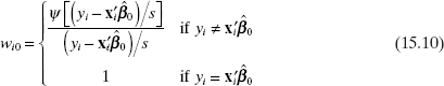
where W₀ is an n × n diagonal matrix of “weights” with diagonal elements w₁₀, w₂₀,…, w_n0 given by Eq. (15.10). We recognize Eq. (15.11) as the usual weighted least-squares normal equations. Consequently, the one-step estimator is

At the next step we recompute the weights from Eq. (15.10) but using instead of . Usually only a few iterations are required to achieve convergence. The iteratively reweighted least-squares procedure could be implemented using a standard weighted least-squares computer program.

A number of popular robust criterion functions are shown in Table 15.1 behavior of these ρ functions and their corresponding ψ functions are illustrated in Figures 15.3 and 15.4, respectively. Robust regression procedures can be classified by the behavior of their ψ function. The ψ function controls the weight given to each residual and (apart from a constant of proportionality) is sometimes called the influence function. For example, the ψ function for least squares is unbounded, and thus least squares tends to be nonrobust when used with data arising from a heavy-tailed distribution. The Huber t function (Huber [1964]) has a monotone ψ function and does not weight large residuals as heavily as least squares. The last three influence functions actually redescend as the residual becomes larger. Ramsay's E_a function (see Ramsay [1977]) is a soft redescender. that is, the ψ function is asymptotic to zero for large |z|. Andrew's wave function and Hampel's 17A function (see Andrews et al. [1972] and Andrews [1974]) are hard redescenders. that is, the ψ function equals zero for sufficiently large |z|. We should note that the ρ functions associated with the redescending ψ functions are nonconvex, and this in theory can cause convergence problems in the iterative estimation procedure. However, this is not a common occurrence. Furthermore, each of the robust criterion functions requires the analyst to specify certain “tuning constants” for the ψ functions. We have shown typical values of these tuning constants in Table 15.1.

TABLE 15.1 Robust Criterion Functions

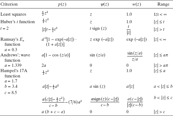
Figure 15.3 Robust criterion functions.

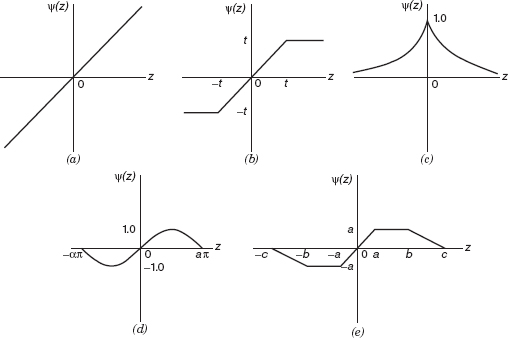
Figure 15.4 Robust influence functions: (a) least squares; (b) Huber's t functions; (c) Ramsay's E_a function; (d) Andrews'; wave function; (e) Hampel's 17A function.

The starting value used in robust estimation can be an important consideration. Using the least-squares solution can disguise the high leverage points. The L₁-norm estimates would be a possible choice of starting values. Andrews [1974] and Dutter [1977] also suggest procedures for choosing the starting values.

It is important to know something about the error structure. of the final robust regression estimates . Determining the covariance matrix of is important if we are to construct confidence intervals or make other model inferences. Huber [1973] has shown that asymptotically has an approximate normal distribution with covariance matrix

Therefore, a reasonable approximation for the covariance matrix of is

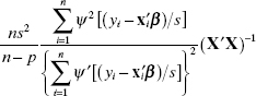
The weighted least-squares computer program also produces an estimate of the covariance matrix

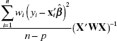
Other suggestions are in Welsch [1975] and Hill [1979]. There is no general agreement about which approximation to the covariance matrix of is best. Both Welsch and Hill note that these covariance matrix estimates perform poorly for X matrices that have outliers. Ill-conditioning (multicollinearity) also distorts robust regression estimates. However, There are indications that in many cases we can make approximate inferences about using procedures similar to the usual normal theory.

Example 15.1 The Stack Loss Data

Andrews [1974] uses the stack loss data analyzed by Daniel and Wood [1980] to illustrate robust regression. The data, which are taken from a plant oxidizing ammonia to nitric acid, are shown in Table 15.2. An ordinary least-squares (OLS) fit to these data gives

TABLE 15.2 Stack Loss Data from Daniel and Wood [1980]

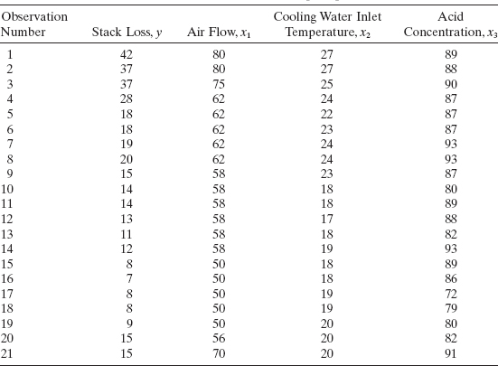
TABLE 15.3 Residuals for Various Fits to the Stack Loss Data^a

The residuals from this model are shown in column 1 of Table 15.3 and a normal probability plot is shown in Figure 15.5a Daniel and Wood note that the residual for point 21 is unusually large and has considerable influence on the regression coefficients. After an insightful analysis, they delete points 1, 3, 4, and 21 from the data, The OLS fit^† to the remaining data yields

The residuals from this model are shown in column 2 of Table 15.3, and the corresponding normal probability plot is in Figure 15.5b. This plot does not indicate any unusual behavior in the residuals.

Andrews [1974] observes that most users of regression lack the skills of Daniel and Wood and employs robust regression methods to produce equivalent results, A robust fit to the stack loss data using the wave function with a = 1.5 yields

Figure 15.5 Normal probability plots from least-squares fits: (a) least squares with all 21 points; (b) least squares with 1, 3, 4, and 21 deleted. (From Andrews [1974], with permission of the publisher.)

This is virtually the same equation found by Daniel and Wood using OLS after much careful analysis, The residuals from this model are shown in column 3 of Table 15.3, and the normal probability plot is in Figure 15.6a. The four suspicious points are clearly identified in this plot Finally, Andrews obtains a robust fit to the data with points 1, 3, 4, and 21 removed. The resulting equation is identical to the one found using all 21 data points, The residuals from this fit and the corresponding normal probability plot are shown in column 4 of Table 15.3 and Figure 15.6b, respectively. This normal probability plot is virtually identical to the one obtained from the OLS analysis with points 1, 3, 4, and 21 deleted (Figure 15.5b)

Once again we find that the routine application of robust regression has led to the automatic identification of the suspicious points. It has also produced a fit that does not depend on these points in any important way. Thus, robust regression methods can be viewed as procedures for isolating unusually influential points, so that these points may be given further study.

Computing M-Estimates Not many statistical software packages compute M-estimates. S-PLUS and STATA do have this capability. SAS recently added it. The SAS code to analyze the stack loss data is:

proc robustreg;
   model y = xl x2 x3 / diagnostics leverage;
run;

SAS's default procedure uses the bisquare weight function (see Problem 15.3) and the median method for estimating the scale parameter.

Robust regression methods have much to offer the data analyst. They can be extremely helpful in locating outliers and highly influential observations. Whenever a least-squares analysis is performed, it would be useful to perform a robust fit also. If the results of the two procedures are in substantial agreement, then use the leasts quares results, because inferences based on least squares are at present better understood. However, if the results of the two analyses differ, then reasons for these differences should be identified. Observations that are downweighted in the robust 0 fit should be carefully examined.

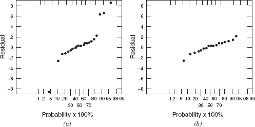
Figure 15.6 Normal probability plots from robust fits: (a) robust fit with all 21 points; (b) robust fit with 1, 3, 4, and 21 deleted. (From Andrews [1974], with permission of the publisher.)

15.1.3 Properties of Robust Estimators

In this section we introduce two important properties of robust estimators: breakdown and efficiency. We will observe that the breakdown point of an estimator is a practical concern that should be taken into account when selecting a robust estimation procedure. Generally, M-estimates perform poorly with respect to breakdown point. This has spurred development of many other alternative procedures.

Breakdown Point The finite-sample breakdown point is the smallest fraction of anomalous data that can cause the estimator to be useless. The smallest possible breakdown point is 1/n, that is, a single observation can distort the estimator so badly that it is of no practical use to the regression model-builder. The breakdown point of OLS is 1/n.

M-estimates can be affected by x-space outliers in an identical manner to OLS. Consequently, the breakdown point of the class of M-estimators is 1/n. This has a potentially serious impact on their practical use, since it can be difficult to determine the extent to which the sample is contaminated with anomalous data. Most experienced data analysts believe that the fraction of data that are contaminated by erroneous data typically varies between 1 and 10%. Therefore, we would generally want the breakdown point of an estimator to exceed 10%. This has led to the development of high-breakdown-point estimators.

Efficiency Suppose that a data set has no gross errors, there are no influential observations, and the observations come from a normal distribution. If we use a robust estimator on such a data set, we would want the results to be virtually identical to OLS, since OLS is the appropriate technique for such data. The efficiency of a robust estimator can be thought of as the residual mean square obtained from OLS divided by the residual mean square from the robust procedure. Obviously, we want this efficiency measure to be close to unity.

There is a lot of emphasis in the robust regression literature on asymptotic efficiency, that is, the efficiency of an estimator as the sample size n becomes infinite. This is a useful concept in comparing robust estimators, but many practical regression problems involve small to moderate sample sizes (n < 50, for instance), and small-sample efficiencies are known to differ dramatically from their asymptotic values. Consequently, a model-builder should be interested in the asymptotic behavior of any estimator that might be used in a given situation but should not be unduly excited about it. What is more important from a practical viewpoint is the finite-sample efficiency, or how well a particular estimator works with reference to OLS on “clean” data for sample sizes consistent with those of interest in the problem at hand. The finite-sample efficiency of a robust estimator is defined as the ratio of the OLS residual mean square to the robust estimator residual mean square, where OLS is applied only to the clean data. Monte Carlo simulation methods are often used to evaluate finite-sample efficiency.

15.2 EFFECT OF MEASUREMENT ERRORS IN THE REGRESSORS

In almost all regression models we assume that the response variable y is subject to the error term ε and that the regressor variables x₁, x₂,…, x_k are deterministic or mathematical variables, not affected by error. There are two variations of this situation. The first is the case where the response and the regressors are jointly distributed random variables This assumption gives rise to the correlation model discussed in Chapter 2 (refer to Section 2.12). The second is the situation where there are measurement errors in the response and the regressors. Now if measurement errors are present only in the response variable y, there are no new problems so long as these errors are uncorrelated and have no bias (zero expectation). However, a different situation occurs when there are measurement errors in the x's. We consider this problem in this section.

15.2.1 Simple Linear Regression

Suppose that we wish to fit the simple linear regression model, but the regressor is measured with error, so that the observed regressor is

where x_i is the true value of the regressor, X_i is the observed value, and a_i is the measurement error with E(a_i) = 0 and Var The response variable y_i is subject to the usual error ε_i, i = 1, 2,…, n, so that the regression model is

We assume that the errors ε_i and a_i are uncorrelated, that is, E(ε_ia_i) = 0. This is sometimes called the errors-in-both-variables model. Since X_i is the observed value of the regressor, we may write

Initially Eq. (15.14) may look like an ordinary linear regression model with error term γ_i = ε_i − β₁a_i. However, the regressor variable X_i is a random variable and is correlated with the error term γ_i = ε_i − β₁a_i. The correlation between X_i and γ_i is easily seen, since

Thus, if β₁ ≠ 0, the observed regressor X_i and the error term γ_i are correlated.

The usual assumption when the regressor is a random variable is that the regressor variable and the error component are independent. Violation of this assumption introduces several complexities into the problem. For example, if we apply standard least-squares methods to the data (i.e., ignoring the measurement error), the estimators of the model parameters are no longer unbiased. In fact, we can show that if Cov(X_i, γ_i) = 0, then

where

That is, is always a biased estimator of β₁ unless which occurs only when there are no measurement errors in the x_i.

Since measurement error is present to some extent in almost all practical regression situations, some advice for dealing with this problem would be helpful. Note that if is small relative to the bias in will be small. This implies that if the variability in the measurement errors is small relative to the variability of the x's, then the measurement errors can be ignored and standard least-squares methods applied.

Several alternative estimation methods have been proposed to deal with the problem of measurement errors in the variables. Sometimes these techniques are discussed under the topics structural or functional relationships in regression. Economists have used a technique called two-stage least squares in these cases. Often these methods require more extensive assumptions or information about the parameters of the distribution of measurement errors. Presentations of these methods are in Graybill [1961], Johnston [1972], Sprent [1969], and Wonnacott and Wonnacott [1970]. Other useful references include Davies and Hutton [1975], Dolby [1976], Halperin [1961], Hodges and Moore [1972], Lindley [1974], Mandansky [1959], and Sprent and Dolby [1980]. Excellent discussions of the subject are also in Draper and Smith [1998] and Seber [1977].

15.2.2 The Berkson Model

Berkson [1950] has investigated a case involving measurement errors in x_i where the method of least squares can be directly applied. His approach consists of setting the observed value of the regressor X_i to a target value. This forces X_i to be treated as fixed, while the true value of the regressor x_i = X_i − a_i becomes a random variable. As an example of a situation where this approach could be used, suppose that the current flowing in an electrical circuit is used as a regressor variable. Current flow is measured with an ammeter, which is not completely accurate, so measurement error is experienced. However, by setting the observed current flow to target levels of 100, 125, 150, and 175 A (for example), the observed current flow can be considered as fixed, and actual current flow becomes a random variable. This type of problem is frequently encountered in engineering and physical science. The regressor is a variable such as temperature, pressure, or flow rate and there is error present in the measuring instrument used to observe the variable. This approach is also sometimes called the controlled-independent-variable model.

If X_i is regarded as fixed at a preassigned target value, then Eq. (15.14), found by using the relationship X_i = x_i + a_i, is still appropriate. However, the error term in this model, γ_i = ε_i – β₁a_i, is now independent of X_i because X_i is considered to be a fixed or nonstochastic variable. Thus, the errors are uncorrelated with the regressor, and the usual least-squares assumptions are satisfied. Consequently, a standard least-squares analysis is appropriate in this case.

15.3 INVERSE ESTIMATION—THE CALIBRATION PROBLEM

Most regression problems involving prediction or estimation require determining the value of y corresponding to a given x, such as x₀ In this section we consider the inverse problem; that is, given that we have observed a value of y, such as y₀, determine the x value corresponding to it. For example, suppose we wish to calibrate a thermocouple, and we know that the temperature reading given by the thermocouple is a linear function of the actual temperature, say

or

Now suppose we measure an unknown temperature with the thermocouple and obtain a reading y₀. We would like to estimate the actual temperature, that is, the temperature x₀ corresponding to the observed temperature reading y₀. This situation arises often in engineering and physical science and is sometimes called the calibration problem. It also occurs in bioassay where a standard curve is constructed against which all future assays or discriminations are to be run.

Suppose that the thermocouple has been subjected to a set of controlled and known temperatures x₁, x₂, …, x_n and a set of corresponding temperature readings y₁, y₂, …, y_n obtained. One method for estimating x given y would be to fit the model (15.15), giving

Now let y₀ be the observed value of y. A natural point estimate of the corresponding value of x is

assuming that This approach is often called the classical estimator.

Graybill [1976] and Seber [1977] outline a method for creating a 100 (1 – α) percent confidence region for x₀. Previous editions of this book did recommend this approach. Parker, et al. [2010] show that this method really does not work well. The actual confidence level is much less than the advertised (1 – α) percent. They establish that the interval based on the delta method works quite well. Let n be the number of data points in the calibration data collection. This interval is

where MS_Res, , and S_xx are all calculated from the data collected from the calibration.

Example 15.2 Thermocouple Calibration

A mechanical engineer is calibrating a thermocouple. He has chosen 16 levels of temperature evenly spaced over the interval 100–400°C. The actual temperature x (measured by a thermometer of known accuracy) and the observed reading on the thermocouple y are shown in Table 15.4 and a scatter diagram is plotted in Figure 15.7] Inspection of the scatter diagram indicates that the observed temperature on the thermocouple is linearly related to the actual temperature. The straight-line model is

with σ² = MS_Res = 5.86. The F statistic for this model exceeds 20,000, so we reject H₀: β₁ = 0 and conclude that the slope of the calibration line is not zero. Residual analysis does not reveal any unusual behavior so this model can be used to obtain point and interval estimates of actual temperature from temperature readings on the thermocouple.

Suppose that a new observation on temperature of y₀ = 200°C is obtained using the thermocouple. A point estimate of the actual temperature, from the calibration line, is

the 95% prediction interval based on (15.18) is 211.21 ≤ x₀ ≤ 222.5

TABLE 15.4 Actual and Observed Temperature

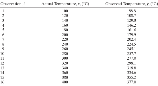
Figure 15.7 Scatterplot of observed and actual temperatures, Example 15.2.

Other Approaches Many peopled o not find the classical procedure outlined in Example 15.2 entirely satisfactory. Williams [1969] claims that the classical estimator has infinite variance based on the assumption that this estimator follows a Cauchy-like distribution. A Cauchy random variable is the inverse of a standard normal random variable. This standard normal random variable has a mean of 0, which does create problems for the Cauchy distribution. The analyst always can rescale the calibration data such that the slope is one. Typically, the variances for calibration experiments are very small, on the order of σ = 0.01. In such a case, the slope for the calibration data is approximately 100 standard deviations away from 0. Williams and similar arguments about infinite variance have no practical import.

The biggest practical complaint about the classical estimator is the difficulty in implementing the procedure. Many analysts, particularly outside the classical laboratory-calibration context, prefer inverse regression, where the analyst treats the xs in the calibration experiment as the response and the ys as the regressor. Of course, this reversal of roles is problematic in itself. Ordinary least squares regression assumes that the regressors are measured without error and that the response is random. Clearly, inverse regression violates this basic assumption.

Krutchkoff [1967, 1969] performed a series of simulations comparing the classical approach to inverse regression. He concluded that inverse regression was a better approach in terms of mean squared error of prediction. However, Berkson [1969], Halperin [1970], and Williams [1969] criticized Krutchkoff's results and conclusions.

Parker et al. [2010] perform a thorough comparison of the classical approach and inverse regression. They show that both approaches yield biased estimates. The bias for the classical estimator is

The bias for inverse regression is approximately

Interestingly, inverse regression suffers from more bias than the classical approach.

Parker et al. conclude that for quite accurate instruments (σ ≈ 0.01), the classical approach and inverse regression yield virtually the same intervals. For borderline instruments (σ ≈ 0.1), inverse regression gives slightly smaller widths. Both procedures yield coverage probabilities as advertised.

A number of other estimators have been proposed. Graybill [1961, 1976] considers the case where we have repeated observations on y at the unknown value of x. He develops point and interval estimates for x using the classical approach. The probability of obtaining a finite confidence interval for the unknown x is greater when those are repeat observations on y. Hoadley [1970] gives a Bayesian treatment of the problem and derives an estimator that is a compromise between the classical and inverse approaches. He notes that the inverse estimator is the Bayes estimator for a particular choice of prior distribution. Other estimators have been proposed by Kalotay [1971], Naszódi [1978], Perng and Tong [1974], and Tucker [1980]. The paper by Scheffé [1973] is also of interest. In genenal, Parker et al. [2010] show that these approaches are not satisfactory since the resulting intervals are very conservative with the actual coverage probability much greater than 100 (1 – α).

In many, if not most, calibration studies the analyst can design the data collection experiment. That is, he or she can specify what x values are to be observed. Ott and Myers [1968] have considered the choice of an appropriate design for the inverse estimation problem assuming that the unknown x is estimated by the classical approach. They develop designs that are optimal in the sense of minimizing the integrated mean square error. Figures are provided to assist the analyst in design selection.

15.4 BOOTSTRAPPING IN REGRESSION

For the standard linear regression model, when the assumptions are satisfied, there are procedures available for examining the precision of the estimated regression coefficients, as well as the precision of the estimate of the mean or the prediction of a future observation at any point of interest. These procedures are the familiar standard errors, confidence intervals, and prediction intervals that we have discussed in previous chapters. However, there are many regression model-fitting situations either where there is no standard procedure available or where the results available are only approximate techniques because they are based on large-sample or asymptotic theory. For example, for ridge regression and for many types of robust fitting procedures there is no theory available for construction of confidence intervals or statistical tests, while in both nonlinear regression and generalized linear models the only tests and intervals available are large-sample results.

Bootstrapping is a computer-intensive procedure that was developed to allow us to determine reliable estimates of the standard errors of regression estimates in situations such as we have just described. The bootstrap approach was originally developed by Efron [1979, 1982]. Other important and useful references are Davison and Hinkley [1997], Efron [1987], Efron and Tibshirani [1986, 1993], and Wu [1986]. We will explain and illustrate the bootstrap in the context of finding the standard error of an estimated regression coefficient. The same procedure would be applied to obtain standard errors for the estimate of the mean response or a future observation on the response at a particular point. Subsequently we will show how to obtain approximate confidence intervals through bootstrapping.

Suppose that we have fit a regression model, and our interest focuses on a particular regression coefficient, say . We wish to estimate the precision of this estimate by the bootstrap method. Now this regression model was fit using a sample of n observations. The bootstrap method requires us to select a random sample of size n with replacement from this original sample. This is called the bootstrap sample. Since it is selected with replacement, the bootstrap sample will contain observations from the original sample, with some of them duplicated and some of them omitted. Then we fit the model to this bootstrap sample, using the same regression procedure as for the original sample. This produces the first bootstrap estimate, say . This process is repeated a large number of times. On each repetition, a bootstrap sample is selected, the model is fit, and an estimate is obtained for i = 1, 2, …, m bootstrap samples. Because repeated samples are taken from the original sample, bootstrapping is also called a resampling procedure. Denote the estimated standard deviation of the m bootstrap estimates by . This bootstrap standard deviation is an estimate of the standard deviation of the sampling distribution of and, consequently, it is a measure of the precision of estimation for the regression coefficient β.

15.4.1 Bootstrap Sampling in Regression

We will describe how bootstrap sampling can be applied to a regression model. For convenience, we present the procedures in terms of a linear regression model, but they could be applied to a nonlinear regression model or a generalized linear model in essentially the same way.

There are two basic approaches for bootstrapping regression estimates. In the first approach, we fit the linear regression model y = X β + ε and obtain the n residuals e′ = [e₁, e₂, …, e_n]. Choose a random sample of size n with replacement from these residuals and arrange them in a bootstrap residual vector e*. Attach the bootstrapped residuals to the predicted values to form a bootstrap vector of responses y*. That is, calculate

These bootstrapped responses are now regressed on the original regressors by the regression procedure used to fit the original model. This produces the first bootstrap estimate of the vector of regression coefficients. We could now also obtain bootstrap estimates of any quantity of interest that is a function of the parameter estimates. This procedure is usually referred to as bootstrapping residuals.

Another bootstrap sampling procedure, usually called bootstrapping cases (or bootstrapping pairs), is often used in situations where there is some doubt about the adequacy of the regression function being considered or when the error variance is not constant and/or when the regressors are not fixed-type variables. In this variation of bootstrap sampling, it is the n sample pairs (x_i, y_i) that are considered to be the data that are to be resampled. That is, the n original sample pairs (x_i, y_i) are sampled with replacement n times, yielding a bootstrap sample, say (x*_i, y*_i) for i = 1, 2, …, n. Then we fit a regression model to this bootstrap sample, say

resulting in the first bootstrap estimate of the vector of regression coefficients.

These bootstrap sampling procedures would be repeated m times. Generally, the choice of m depends on the application. Sometimes, reliable results can be obtained from the bootstrap with a fairly small number of bootstrap samples. Typically, however, 200–1000 bootstrap samples are employed. One way to select m is to observe the variability of the bootstrap standard deviation as m increases. When stabilizes, a bootstrap sample of adequate size has been reached.

15.4.2 Bootstrap Confidence Intervals

We can use bootstrapping to obtain approximate confidence intervals for regression coefficients and other quantities of interest, such as the mean response at a particular point in x space, or an approximate prediction interval for a future observation on the response. As in the previous section, we will focus on regression coefficients, as the extension to other regression quantities is straightforward.

A simple procedure for obtaining an approximate 100(1 – α) percent confidence interval through bootstrapping is the reflection method (also known as the percentile method). This method usually works well when we are working with an unbiased estimator. The reflection confidence interval method uses the lower 100(α/2) and upper 100(1 – α/2) percentiles of the bootstrap distribution of . Let these percen tiles be denoted by and respectively. Operationally, we would obtain these percentiles from the sequence of bootstrap estimates that we have computed, Define the distances of these percentiles from , the estimate of the regression coefficient obtained for the original sample, as follows:

Then the approximate 100(1 – α/2) percent bootstrap confidence interval for the regression coefficient β is given by

Before presenting examples of this procedure, we note two important points:

1. When using the reflection method to construct bootstrap confidence intervals, it is generally a good idea to use a larger number of bootstrap samples than would ordinarily be used to obtain a bootstrap standard error. The reason is that small tail percentiles of the bootstrap distribution are required, and a larger sample will provide more reliable results. Using at least m = 500 bootstrap samples is recommended.
2. The confidence interval expression in Eq. (15.22) associates D₂ with the lower confidence limit and D₁ with the upper confidence limit, and at first glance this looks rather odd since D₁ involves the lower percentile of the bootstrap distribution and D₂ involves the upper percentile. To see why this is so, consider the usual sampling distribution of for which the lower 100(α/2) and upper 100(1 – α/2) percentiles are denoted by and respectively. Now we can state with probability 100(1 – α/2) that will fall in the interval

   

   Expressing these percentiles in terms of the distances from the mean of the sampling distribution of , that is, we obtain

   

   Therefore,

   

   Substituting Eq. (15.24) into Eq. (15.23) produces

   

   which can be written as

   

   this last equation is of the same form as the bootstrap confidence interval, Eq. (15.22), with D₁ and D₂ replacing d₁, and d₂ and using as an estimate of the mean of the sampling distribution.

We now present two examples. In the first example, standard methods are available for constructing the confidence interval, and our objective is to show that similar results are obtained by bootstrapping. The second example involves nonlinear regression, and the only confidence interval results available are based on asymptotic theory. We show how the bootstrap can be used to check the adequacy of the asymptotic results.

Example 15.3 The Delivery Time Data

The multiple regression version of these data, first introduced in Example 3.1 has been used several times throughout the book to illustrate various regression techniques. We will show how to obtain a bootstrap confidence interval for the regression coefficient for the predictor cases, β₁. From Example 3.1, the least-squares estimate of β₁ is In Example 3.8 we found that the standard error of is 0.17073, and the 95% confidence interval for β₁ is 1.26181 ≤ β₁≤ 1.97001.

Since the model seems to fit the data well, and there is not a problem with inequality of variance, we will bootstrap residuals to obtain an approximate 95% bootstrap confidence interval for β₁. Table 3.3 shows the fitted values and residuals for all 25 observations based on the original least-squares fit. To construct the first bootstrap sample, consider the first observation. The fitted value for this observation is ŷ₁ = 21.7081, from Table 3.3. Now select a residual at random from the last column of this table, say e₅ = −0.4444. This becomes the first bootstrap residual e₁^* = −0.4444. Then the first bootstrap observation becomes y₁^* = y₁ + e₁^* = 21.7081–0.4444 = 21.2637. Now we would repeat this process for each subsequent observation using the fitted values ŷ_i and the bootstrapped residuals e_i^* for i = 2, 3, …, 25 to construct the remaining observations in the bootstrap sample. Remember that the residuals are sampled from the last column of Table 3.3 with replacement. After the bootstrap sample is complete, fit a linear regression model to the observations (x_i1, x_i2, y_i*), i = 2 3, …, 25. The result from this yields the first bootstrap estimate of the regression coefficient, We repeated this process m = 1000 times, producing 1000 bootstrap estimates Figure 15.8 shows the histogram of these bootstrap estimates. Note that the shape of this histogram closely resembles the normal distribution. This is not unexpected, since the sampling distribution of should be a normal distribution. Furthermore, the standard deviation of the 1000 bootstrap estimates is which is reasonably close to the usual normal-theory-based standard error of , se

To construct the approximate 95% bootstrap confidence interval for , we need the 2.5th and 97.5th percentiles of the bootstrap sampling distribution. These quantities are and respectively (refer to Figure 15.8). The distances D₁ and D₂ are computed from Eq. (15.21) as follows:

Finally, the approximate 95% bootstrap confidence interval is obtained from Eq.

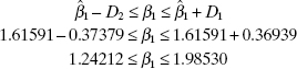
This is very similar to the exact normal-theory confidence interval found in Example 3.8, 1.26181 ≤ β₁ ≤ 1.97001. We would expect the two confidence intervals to closely agree, since there is no serious problem here with the usual regression assumptions.

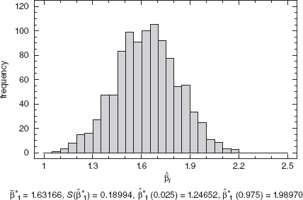
Figure 15.8 Histogram of bootstrap , Example 15.3.

The most important applications of the bootstrap in regression are in situations either where there is no theory available on which to base statistical inference or where the procedures utilize large-sample or asymptotic results. For example, in nonlinear regression, all the statistical tests and confidence intervals are large-sample procedures and can only be viewed as approximate procedures. In a specific problem the bootstrap could be used to examine the validity of using these asymptotic procedures.

Example 15.4 The Puromycin date

Examples 12.2 and 12.3 introduced the puromycin data, and we fit the Michaelis-Menten model

to the data in Table 12.1 which resulted in estimates of and respectively. We also found the large-sample standard errors for these parameter estimates to be se and se and the approximate 95% confidence intervals were computed in Example 12.6 as

and

Since the inference procedures used here are based on large-sample theory, and the sample size used to fit the model is relatively small (n = 12), it would be useful to check the validity of applying the asymptotic results by computing bootstrap standard deviations and bootstrap confidence intervals for θ₁ and θ₂. Since the Michaelis-Menten model seems to fit the data well, and there are no significant problems with inequality of variance, we used the approach of bootstrapping residuals to obtain 1000 bootstrap samples each of size n = 12. Histograms of the resulting bootstrap estimates of θ₁ and θ₂ are shown in Figures 15.9 and 15.10, respectively. The sample average, standard deviation, and 2.5th and 97.5th percentiles are also shown for each bootstrap distribution. Notice that the bootstrap averages and standard deviations are reasonably close to the values obtained from the original non-linear least-squares fit. Furthermore, both histograms are reasonably normal in appearance, although the distribution for may be slightly skewed.

We can calculate the approximate 95% confidence intervals for θ₁ and θ₂. Consider first θ₁. From Eq. (15.21) and the information in Figure 15.9 we find

Therefore, the approximate 95% confidence interval is found from Eq. (15.22) as follows:

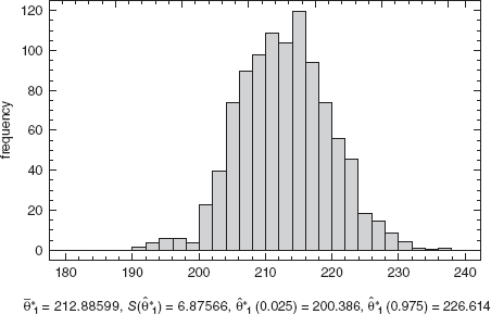
Figure 15.9 Histogram of bootstrap estimates , Example 15.4.

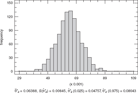
Figure 15.10 Histogram of bootstrap estimates , Example 15.4.

This is very close to the asymptotic normal-theory interval calculated in the original problem. Following a similar procedure we obtain the approximate 95% bootstrap confidence interval for θ₂ as

Once again, this result is similar to the asymptotic normal-theory interval calculated in the original problem. This gives us some assurance that the asymptotic results apply, even though the sample size in this problem is only n = 12.

15.5 CLASSIFICATION AND REGRESSION TREES (CART)

The general classification problem can be stated as follows: given a response of interest and certain taxonomic data (measurement data or categorical descriptors) on a collection of units, use these data to predict the “class” into which each unit falls. The algorithm for accomplishing this task can then be used to make predictions about future units where the taxonomic data are known but the response is not. This is, of course, a very general problem, and many different statistical tools might be applied to it, including standard multiple regression, logistic regression or generalized linear models, cluster analysis, discriminant analysis, and so forth. In recent years, statisticians and computer scientists have developed tree-based algorithms for the classification problem. We give a brief introduction to these techniques in this section. For more details, see Breiman, Friedman, Olshen, and Stone [1984] and Gunter [1997a,b, 1998].

When the response variable is discrete, the procedure is usually called classification, and when it is continuous, the procedure leads to a regression tree. The usual acronym for the algorithms that perform these procedures is CART, which stands for classification and regression trees. A classification or regression tree is a hierarchical display of a series of questions about each unit in the sample. These questions relate to the values of the taxonomic data on each unit. When these questions are answered, we will know the “class” to which each unit most likely belongs. The usual display of this information is called a tree because it is logical to represent the questions as an upside-down tree with a root at the top, a series of branches connecting nodes, and leaves at the bottom. At each node, a question about one of the taxonomic variables is posed and the branch taken at the node depends on the answer. Determining the order in which the questions are asked is important, because it determines the structure of the tree. While there are many ways of doing this, the general principle is to ask the question that maximizes the gain in node purity at each node-splitting opportunity, where node purity is improved by minimizing the variability in the response data at the node. Thus, if the response is a discrete classification, higher purity would imply fewer classes or categories. A node containing a single class or category of the response would be completely pure. If the response is continuous, then a measure of variability such as a standard deviation, a mean square error, or a mean absolute deviation of the responses at a node should be made as small as possible to maximize node purity.

There are numerous specific algorithms for implementing these very general ideas, and many different computer software codes are available. CART techniques are often applied to very large or massive data sets, so they tend to be very computer intensive. There are many applications of CART techniques in situations ranging from interpretation of data from designed experiments to large-scale data exploration (often called data mining, or knowledge discovery in data bases).

Example 15.5 The Gasoline Mileage Data

Table B.3 presents gasoline mileage performance data on 32 automobiles, along with 11 taxonomic variables. There are missing values in two of the observations, so we will confine our analysis to only the 30 vehicles for which complete samples are available. Figure 15.11 presents a regression tree produced by S-PLUS applied to this data set. The bottom portion of the figure shows the descriptive information (also in hierarchical format) produced by S-PLUS for each node in the tree. The measure of node purity or deviance at each node is just the corrected sum of squares of the observations at that node, yval is the average of these observations, and n refers to the number of observations at the node.

At the root node, we have all 30 cars, and the deviance there is just the corrected sum of squares of all 30 cars. The average mileage in the sample is 20.04 mpg. The first branch is on the variable CID, or cubic inches of engine displacement. There are four cars in node 2 that have a CID below 115.25, their deviance is 22.55, and the average mileage performance is 33.38 mpg. The deviance in node 3 from the right-hand branch of the root node is 295.6 and the sum of the deviances from nodes 2 and 3 is 318.15. There are no other splits possible at any level on any variable to classify the observations that will result in a lower sum of deviances than 318.15.

Figure 15.11 CART analysis from S-PLUS for the gasoline mileage data from Table B.3.

Node 2 is a terminal node because the node deviance is a smaller percentage of the root node deviance than the user specified allowance. Terminal nodes can also occur if there are not enough observations (again, user specified) to split the node. So, at this point, if one wishes to identify cars in the highest-mileage performance group, all we need to look at is engine displacement.

Node 3 contains 26 cars, and it is subsequently split at the next node by horse-power. Eleven cars with horsepower below 141.5 form one branch from this node, while 15 cars with horsepower above 141.5 form the other branch. The left-hand branch results in the terminal node 6. The right-hand branch enters another node (7) which is branched again on horsepower. This illustrates an important feature of regression trees; the same question can be asked more than once at different nodes of the tree, reflecting the complexity of the interrelationships among the variables in the problem. Nodes 14 and 15 are terminal nodes, and the cars in both terminal nodes have similar mileage performance.

The tree indicates that we may be able to classify cars into higher-mileage, medium-mileage, and lower-mileage classifications by examining CID and horsepower—only 2 of the 11 taxonomic variables given in the original data set. For purposes of comparison, forward variable selection using mpg as the response would choose CID as the only important variable, and either stepwise regression or back-ward elimination would select rear axle ratio, length, and weight. However, remember that the objectives of CART and multiple regression are somewhat different: one is trying to find an optimal (or near-optimal) classification structure, while the other seeks to develop a prediction equation.

15.6 NEURAL NETWORKS

Neural networks, or more accurately artificial neural networks, have been motivated by the recognition that the human brain processes information in a way that is fundamentally different from the typical digital computer. The neuron is the basic structural element and information-processing module of the brain. A typical human brain has an enormous number of them (approximately 10 billion neurons in the cortex and 60 trillion synapses or connections between them) arranged in a highly complex, nonlinear, and parallel structure. Consequently, the human brain is a very efficient structure for information processing, learning, and reasoning.

An artificial neural network is a structure that is designed to solve certain types of problems by attempting to emulate the way the human brain would solve the problem. The general form of a neural network is a “black-box” type of model that is often used to model high-dimensional, nonlinear data. Typically, most neural networks are used to solve prediction problems for some system, as opposed to formal model building or development of underlying knowledge of how the system works. For example, a computer company might want to develop a procedure for automatically reading handwriting and converting it to typescript. If the procedure can do this quickly and accurately, the company may have little interest in the specific model used to do it.

Multilayer feedforward artificial neural networks are multivariate statistical models used to relate p predictor variables x₁, x₂, …, x_p to q response variables y₁, y₂, …, y_q. The model has several layers, each consisting of either the original or some constructed variables. The most common structure involves three layers: the inputs, which are the original predictors; the hidden layer, comprised of a set of constructed variables; and the output layer, made up of the responses. Each variable in a layer is called a node. Figure 15.12 shows a typical three-layer artificial neural network.

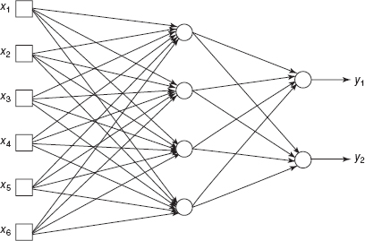
Figure 15.12 Artificial neural network with one hidden layer.

A node takes as its input a transformed linear combination of the outputs from the nodes in the layer below it. Then it sends as an output a transformation of itself that becomes one of the inputs, to one or more nodes on the next layer. The transformation functions are usually either sigmoidal (S shaped) or linear and are usually called activation functions or transfer functions. Let each of the k hidden layer nodes a_u be a linear combination of the input variables:

where the w_1ju are unknown parameters that must be estimated (called weights) and θ_u is a parameter that plays the role of an intercept in linear regression (this parameter is sometimes called the bias node).

Each node is transformed by the activation function g(). Much of the neural networks literature refers to these activation functions notationally as σ() because of their S shape (this is an unfortunate choice of notation so far as statisticians are concerned). Let the output of node a_u be denoted by Z_u = g(a_u). Now we form a linear combination of these outputs, say , where z₀ = 1. Finally, the νth response y is a transformation of the b, say where is the activation function for the response. This can all be combined to give

The response y_ν is a transformed linear combination of transformed linear combinations of the original predictors. For the hidden layer, the activation function is often chosen to be either the logistic function g(x) = 1/(1 + e^−x) or the hyperbolic tangent function g(x) = tanh(x) = (e^x – e^−x)/(e^x + e^−x). The choice of activation function for the output layer depends on the nature of the response. If the response is bounded or dichotomous, the output activation function is usually taken to be sigmoidal, while if it is continuous, an identify function is often used.

The model in Eq. (15.25) is a very flexible form containing many parameters, and it is this feature that gives a neural network a nearly universal approximation property. That is, it will fit many naturally occurring functions. However, the parameters in Eq. (15.25) must be estimated, and there are a lot of them. The usual approach is to estimate the parameters by minimizing the overall residual sum of squares taken over all responses and all observations. This is a nonlinear least-squares problem, and a variety of algorithms can be used to solve it. Often a procedure called backpropagation (which is a variation of steepest descent) is used, although derivative-based gradient methods have also been employed. As in any nonlinear estimation procedure, starting values for the parameters must be specified in order to use these algorithms. It is customary to standardize all the input variables, so small essentially random values are chosen for the starting values.

With so many parameters involved in a complex nonlinear function, there is considerable danger of overfitting. That is, a neural network will provide a nearly perfect fit to a set of historical or “training” data, but it will often predict new data very poorly. Overfilling is a familiar problem to statisticians trained in empirical model building. The neural network community has developed various methods for dealing with this problem, such as reducing the number of unknown parameters (this is called “optimal brain surgery”), stopping the parameter estimation process before complete convergence and using cross-validation to determine the number of iterations to use, and adding a penalty function to the residual sum of squares that increases as a function of the sum of the squares of the parameter estimates. There are also many different strategies for choosing the number of layers and number of neurons and the form of the activation functions. This is usually referred to as choosing the network architecture. Cross-validation can be used to select the number of nodes in the hidden layer. Good references on artificial neural networks are Bishop [1995], Haykin [1994], and Ripley [1994].

Artificial neural networks are an active area of research and application, particularly for the analysis of large, complex, highly nonlinear problems. The overfilling issue is frequently overlooked by many users and advocates of neural networks, and because many members of the neural network community do not have sound training in empirical model building, they often do not appreciate the difficulties overfitting may cause. Furthermore, many computer programs for implementing neural networks do not handle the overfitting problem particularly well. Our view is that neural networks are a complement to the familiar statistical tools of regression analysis and designed experiments and not a replacement for them, because a neural network can only give a prediction model and not fundamental insight into the underlying process mechanism that produced the data.

15.7 DESIGNED EXPERIMENTS FOR REGRESSION

Many properties of the fitted regression model depend on the levels of the predictor variables. For example, the X′X matrix determines the variances and covariances of the model regression coefficients. Consequently, in situations where the levels of the x's can be chosen it is natural to consider the problem of experimental design. That is, if we can choose the levels of each of the predictor variables (and even the number of observations to use), how should we go about this? We have already seen an example of this in Chapter 5 on fitting polynomials where a central composite design was used to fit a second-order polynomial in two variables. Because many problems in engineering, business, and the sciences use low-order polynomial models (typically first-order and second-order polynomials) in their solution there is an extensive literature on experimental designs for fitting these models. For example, see the book on experimental design by Montgomery (2009) and the book on response surface methodology by Myers, Montgomery, and Anderson-Cook (2009). This section gives an overview of designed experiments for regression models and some useful references.

Suppose that we want to fit a first-order polynomial in three variables, say,

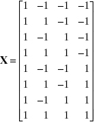
and we can specify the levels of the three regressor variables. Assume that the regressor variables are continuous and can be varied over the range from −1 to +1; that is, −1 ≤ x_i +1, i = 1,2,3. Factorial designs are very useful for fitting regression models. By a factorial design we mean that every possible level of a factor is run in combination with every possible level of all other factors. For example, suppose that we want to run each of the regressor variables at two levels, −1 and +1. Then the factorial design is called a 2³ factorial design and it has n = 8 runs. The design matrix D is just an 8 × 3 matrix containing the levels of the regressors:

The X matrix (or model matrix) is

and the X′X matrix is

Notice that the X′X matrix is diagonal, indicating that the 2³ factorial design is orthogonal. The variance of any regression coefficient is

Furthermore, there is no other eight-run design on the design space bounded by ±1 that would make the variance of the model regression coefficients smaller.

For the 2³ design, the determinant of the X′X matrix is |X′X| = 4096. This is the maximum possible value of the determinant for an eight-run design on the design space bounded by ±1. It turns out that the volume of the joint confidence region that contains all the model regression coefficients is inversely proportional to the square root of the determinant of X′X. Therefore, to make this joint confidence region as small as possible, we would want to choose a design that makes the determinant of X′X as large as possible. This is accomplished by choosing the 2³ design.

These results generalize to the case of a first-order model in k variables, or a first-order model with interaction. A 2^k factorial design (i.e., a factorial design with all k factors at two levels (±1)) will minimize the variance of the regression coefficients and minimize the volume of the joint confidence region on all of the model parameters. A design with this property is called a D-optimal design. Optimal designs resulted from the work of Kiefer (1959, 1961) and Kiefer and Wolfowitz (1959). Their work is couched in a measure theoretic framework in which an experimental design is viewed in terms of design measure. Design optimality moved into the practical arena in the 1970s and 1980s as designs were put forth as being efficient in terms of criteria inspired by Kiefer and his coworkers. Computer algorithms were developed that allowed “optimal” designs to be generated by a computer package based on the practitioner's choice of sample size, model, ranges on variables, and other constraints.

Now consider the variance of the predicted response for the first-order model in the 2³ design

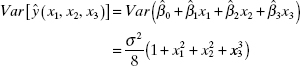
The variance of the predicted response is a function of the point in the design space where the prediction is made (x₁, x₂, and x₃) and the variance of the model regression coefficients. The estimates of the regression coefficients are independent because the 2³ design is orthogonal and the model parameters all have variance σ²/8. Therefore, the maximum prediction variance occurs when x₁ = x₂ = x₃ = ±1 and is equal to σ²/2.

To determine how good this is, we need to know the best possible value of prediction variance that can be attained. It turns out that the smallest possible value of the maximum prediction variance over the design space is pσ²/n, where p is the number of model parameters and n is the number of runs in the design. The 2³ design has n = 8 runs and the model has p = 4 parameters, so the model that we fit to the data from this experiment minimizes the maximum prediction variance over the design region. A design that has this property is called a G-optimal design. In general, 2^k designs are G-optimal designs for fitting the first-order model or the first-order model with interaction.

We can evaluate the prediction variance at any point of interest in the design space. For example, when we are at the center of the design where x₁ = x₂ = x₃ = 0, the prediction variance is

and when x₁ = 1, x₂ = x₃ = 0, the prediction variance is

The average prediction variance at these two points is

A design that minimizes the average prediction variance over a selected set of points is called a V-optimal design.

An alternative to averaging the prediction variance over a specific set of points in the design space is to consider the average prediction variance over the entire design space. One way to calculate this average prediction variance or the integrated variance is

where A is the area or volume of the design space and R is the design region. To compute the average, we are integrating the variance function over the design space and dividing by the area or volume of the region. Now for a 2³ design, the volume of the design region is 8, and the integrated variance is

It turns out that this is the smallest possible value of the average prediction variance that can be obtained from an eight-run design used to fit a first-order model on this design space. A design with this property is called an I-optimal design. In general, 2^k designs are I-optimal designs for fitting the first-order model or the first-order model with interaction.

Now consider designs for fitting second-order polynomials. As we noted in Chapter 7, second-order polynomial models are widely used in industry in the application of response surface methodology (RSM), a collection of experimental design, model fitting, and optimization techniques that are widely used in process improvement and optimization. The second-order polynomial in k factors is

This model has 1 + 2k + k(k – 1)/2 parameters, so the design must contain at least this many runs. In Section 7.4 we illustrated designing an experiment to fit a second-order model in k = 2 factors and the associated model fitting and analysis typical of most RSM studies.

There are a number of standard designs for fitting second-order models. The two most widely used designs are the central composite design and the Box-Behnken design. The central composite design was used in Section 7.4. A central composite design consists of a 2^k factorial design (or a fractional factorial that will allow estimation of all of the second-order model terms), 2k axial runs, defined as follows:

Figure 15.13 The central composite design for k = 2 and .

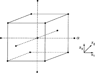
Figure 15.14 The central composite design for k = 3 and .

and n_C center runs at x₁ = x₂ = ··· = x_k = 0. There is considerable flexibility in the use of the central composite design because the experimenter can choose both the axial distance α and the number of center runs. The choice of these two parameters can be very important. Figures 15.13 and 15.14 show the CCD for k = 2 and k = 3. The value of the axial distance generally varies from 1.0 to , the former placing all of the axial points on the face of the cube or hypercube producing a design on a cuboidal region, the latter resulting in all points being equidistant from the design center producing a design on a spherical region. When α = 1 the central composite design is usually called a face-centered cube design. As we observed in Section 7.4, when the axial distance , where F is the number of factorial design points, the central composite design is rotatable; that is, the variance of the predicted response Var[ŷ(x)] is constant for all points that are the same distance from the design center. Rotatability is a desirable property when the model fit to the data from the design is going to be used for optimization. It ensures that the variance of the predicted response depends only on the distance of the point of interest from the design center and not on the direction. Both the central composite design and the Box–Behnken design also perform reasonably well relative to the D-optimality and I-optimality criteria.

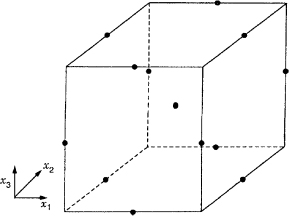
Figure 15.15 The Box–Behnken design for k = 3 factors with one center point.

The Box–Behnken design is also a spherical design that is either rotatable or approximately rotatable. The Box–Behnken design for k = 3 factors is shown in Figure 15.15. All of the points in this design are on the surface of a sphere of radius . Refer to Montgomery (2009) or Myers, Montgomery, and Anderson-Cook (2009) for additional details of central composite and Box–Behnken designs as well as information on other standard designs for fitting the second-order polynomial model.

The JMP software will construct D-optimal and I-optimal designs. The approach used is based on a coordinate exchange algorithm developed by Meyer and Nachtsheim (1995). The experimenter specifies the number of factors, the model that is to be fit, the number of runs in the design, any constraints or restrictions on the design region, and the optimality criterion to be used (D or I). The coordinate exchange technique begins with a randomly chosen design and then systematically searches over each coordinate of each run to find a setting for that coordinate that produces the best value of the criterion. When the search is completed on the last run, it begins again with the first coordinate of the first run. This is continued until no further improvement in the criterion can be made. Now it is possible that the design found by this method is not optimal because ii may depend on the random starting design, so another random design is created and the coordinate exchange process repeated. After several random starts the best design found is declared optimal. This algorithm is extremely efficient and usually produces optimal or very near optimal designs.

To illustrate the construction of optimal designs suppose that we want to run an experiment to fit a second-order model in k = 4 factors. The region of interest is cuboidal and all four factors are defined to be in the interval from −1 to +1. This model has p = 15 parameters, so the design must have at least 15 runs. The central composite design in k = 4 factors has between 25 and 30 runs, depending on the number of center points. This is a relatively large design in comparison to the number of parameters that must be estimated. A fairly typical use of optimal designs is to create a custom design in situations where resources do not permit using the number of runs associated with a standard design. We will construct optimal designs with 18 runs. The 18-run D-optimal design constructed using JMP is shown in Table 15.5, and the I-optimal design is shown in Table 15.6. Both of these designs look somewhat similar. JMP reports the D-efficiency of the design in Table 15.5 as 44.98232% and the D-efficiency of the design in Table 15.6 as 39.91903%. Note that the D-optimal design algorithm did not produce a design with 100% D-efficiency, because the D-efficiency is computed relative to a “theoretical” orthogonal design that may not exist. The G-efficiency for the design in Table 15.5 is 75.38478% and for the design in Table 15.6 it is 73.57805%. The G-efficiency of a design is easy to calculate, because as we observed earlier the theoretical minimum value of the maximum value of the scaled prediction variance over the design space design space is pσ²/n, where p is the number of model parameters and n is the number of runs in the design, so all we have to do is find the actual maximum value of the prediction variance, and the G-efficiency can be calculated from

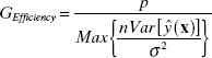
TABLE 15.5 An 18 Run D-Optimal Design for a Second-Order Model in k = 4 Factors

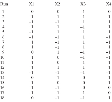
Typically, efficiencies are reported on a percentage basis. Both designs have very similar G-efficiencies. JMP also reports the average (integrated) prediction variance over the design space as 0.652794 σ² for the D-optimal design and 0.48553 σ² for the I-optimal design. It is not surprising that the integrated variance is smaller for the I-optimal design as it was constructed to minimize this quantity.

TABLE 15.6 An 18 Run I-Optimal Design for a Second-Order Model in k = 4 Factors

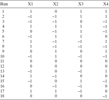
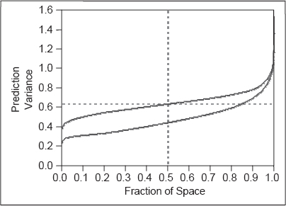
Figure 15.16 Fraction of design space plot for the D-optimal and I-optimal designs in Tables 15.5 and 15.6.

To further compare these two designs, consider the graph in Figure 15.16. This is a fraction of design space (FDS) plot. For any value of prediction variance on the vertical scale the curve shows the fraction or proportion of the total design space in which the prediction variance is less than or equal to the vertical scale value. An “ideal” design would have a low, flat curve on the FDS plot. The lower curve in Figure 15.16 is the I-optimal design and the upper curve is for the D-optimal design. Obviously, the I-optimal design outperforms the D-optimal design in terms of prediction variance over almost all of the design space. It does have a lower G-efficiency, indicating that there is a very small portion of the design space where the maximum prediction variance for the D-optimal design is less than the prediction variance for the I-optimal design. That point is at the extreme end of the region.

PROBLEMS

15.1 Explain why an estimator with a breakdown point of 50% may not give satisfactory results in fitting a regression model.

15.2 Consider the continuous probability distribution f(x). Suppose that θ is an unknown location parameter and that the density may be written as f(x – θ) for –∞ < θ < ∞. Let x₁, x₂, …, x_n be a random sample of size n from the density.

1. Show that the maximum-likelihood estimator of θ is the solution to

   

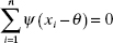
   that maximizes the logarithm of the likelihood function In , where ψ(x) = ρ′(x) and ρ′(x) = –ln f(x).

2. If f(x) is a nonmal distribution, find ρ(x), ψ (x) and the corresponding maximum-likelihood estimator of θ.
3. If f(x) = (2σ)⁻¹e⁻|^x|^/σ (the double-exponential distribution), find ρ(x) and ψ (x). Show that the maximum-likelihood estimator of θ is the sample median. Compare Ibis estimator with the estimator found in part b. Does the sample median seem to be a reasonable estimator in this case?
4. If f(x) = [π (1 + x²)]⁻¹ (the Cauchy distribution), find ρ(x) and ψ (x). How would you solve in this case?

15.3 Tukey's Biwelght. A popular ψ function for robust regression is Tukey's biweight, where

with a = 5, 6 Sketch the ψ function for a = 5 and discuss its behavior. Do you think that Tukey's biweight would give results similar to Andrews' wave function?

15.4 The U.S. Air Force uses regression models for cost estimating, an application that almost always involves outliers. Simpson and Montgomery [1998a] present 19 observations on first-unit satellite cost data (y) and the weight of the electronics suite (x). The data are shown in the following table.

1. Draw a scatter diagram of the data. Discuss what types of outliers may be present.
2. Fit a straight line to these data with OLS. Does this fit seem satisfactory?
3. Fit a straight line to these data with an M-estimator of your choice. Is the fit satisfactory? Discuss why the M-estimator is a poor choice for this problem.
4. Discuss the types of estimators that you think might be appropriate for this data set.

15.5 Table B.14 presents data on the transient points of an electronic inverter. Fit a model to those data using an M-estimator. Is there an indication that observations might have been incorrectly recorded?

15.6 Consider the regression model in Problem 2.10 relating systolic blood pressure to weight. Suppose that we wish to predict an individual's weight given an observed value of systolic blood pressure. Can this be done using the procedure for predicting x given a value of y described in Section 15.3? In this particular application, how would you respond to the suggestion of building a regression model relating weight to systolic blood pressure?

15.7 Consider the regression model in Problem 2.4 relating gasoline mileage to engine displacement.

1. If a particular car has an observed gasoline mileage of 17 miles per gallon, find a point estimate of the corresponding engine displacement.
2. Find a 95% confidence interval on engine displacement.

15.8 Consider a regression model relating total heat flux to radial deflection for the solar energy data in Table B.2.

1. Suppose that the observed total heat flux is 250?kW. Find a point estimate of the corresponding radial deflection.
2. Construct a 90% confidence interval on radial deflection.

15.9 Consider the soft drink delivery time data in Example 3.1. Find an approximate 95% bootstrap confidence interval on the regression coefficient for distance using m = 1000 bootstrap samples. Compare this to the usual normal-theory confidence interval.

15.10 Consider the soft drink delivery time data in Example 3.1. Find the bootstrap estimate of the standard deviation of using the following numbers of bootstrap samples: m = 100, m = 200, m = 300, m = 400, and m = 500. Can you draw any conclusions about how many bootstrap samples are necessary to obtain a reliable estimate of the precision of estimation for

15.11 Describe how you would find a bootstrap estimate of the standard deviation of the estimate of the mean response at a particular point, say x₀.

15.12 Describe how you would find an approximate bootstrap confidence interval on the mean response at a particular point, say x₀.

15.13 Consider the nonlinear regression model fit to the data in Problem 12.11. Find the bootstrap standard errors for the regression coefficients , , and using m = 1000 bootstrap samples. Based on the results you obtain, comment on how the asymptotic theory seems to apply to this problem.

15.14 Consider the nonlinear regression model fit to the data in Problem 12.11. Find approximate 95% bootstrap confidence intervals for the regression coefficients , , and using m = 1000 bootstrap samples. Compare these intervals to the ones based on the large-sample results. Based on the comparison of these intervals, comment on how the asymptotic theory seems to apply to this problem.

15.15 Consider the NFL team performance data in Table B.1. Construct a regression tree for this data set.

15.16 A Designed Experiment for Linear Regression. You wish to fit a simple linear regression model over the region −1 ≤ x ≤ 1 using n = 10 observations. Four experimental designs are under consideration: (i) 5 observations at x = −1 and 5 observations at x = +1, (ii) 4 observations at x = −1, 2 observations at x = 0, and 4 observations at x = +1, (iii) 2 observations at and +1, and (iv) 1 observation at x = −1, −0.8,−0.6, −0.4, −0.2, +0.2, +0.4, +0.6, +0.8, and +1. For each of these designs, find the number of degrees of freedom available for evaluating pure error and testing lack of fit, the standard error of the slope (up to a constant σ), and the value of the determinant of X′X. Based on these analyses, which design would you select?

15.17 An analyst is fitting a simple linear regression model with the objective of obtaining a minimum-variance estimate of the intercept β₀. How should the data collection experiment be designed?

15.18 Suppose that you are fitting a simple linear regression model that will be used to predict the mean response at a particular point such as x₀. How should the data collection experiment be designed so that a minimum-variance estimate of the mean of y at x₀ is obtained?

15.19 Consider the linear regression model y = β₀ + β₁x₁ + β₂x₂ + ε, where the regressors have been coded so that

1. Show that an orthogonal design (X′X diagonal) minimizes the variance of and .
2. Show that any design for fitting this first-order model that is orthogonal is also rotatable.