
CHAPTER 7
POLYNOMIAL REGRESSION MODELS
7.1 INTRODUCTION
The linear regression model y = Xβ + ε is a general model for fitting any relationship that is linear in the unknown parameters β. This includes the important class of polynomial regression models. For example, the second-order polynomial in one variable
![]()
and the second-order polynomial in two variables
![]()
are linear regression models.
Polynomials are widely used in situations where the response is curvilinear, as even complex nonlinear relationships can be adequately modeled by polynomials over reasonably small ranges of the x's. This chapter will survey several problems and issues associated with fitting polynomials.
7.2 POLYNOMIAL MODELS IN ONE VARIABLE
7.2.1 Basic Principles
As an example of a polynomial regression model in one variable, consider

Figure 7.1 An example of a quadratic polynomial.
This model is called a second-order model in one variable. It is also sometimes called a quadratic model, since the expected value of y is
![]()
which describes a quadratic function. A typical example is shown in Figure 7.1. We often call β1 the linear effect parameter and β2 the quadratic effect parameter. The parameter β0 is the mean of y when x = 0 if the range of the data includes x = 0. Otherwise β0 has no physical interpretation.
In general, the kth-order polynomial model in one variable is
If we set xj = xj, j = 1, 2, …, k, then Eq. (7.2) becomes a multiple linear regression model in the k regressors x1, x2, … xk. Thus, a polynomial model of order k may be fitted using the techniques studied previously.
Polynomial models are useful in situations where the analyst knows that curvilinear effects are present in the true response function. They are also useful as approximating functions to unknown and possibly very complex nonlinear relationships. In this sense, the polynomial model is just the Taylor series expansion of the unknown function. This type of application seems to occur most often in practice.
There are several important considerations that arise when fitting a polynomial in one variable. Some of these are discussed below.
- Order of the Model It is important to keep the order of the model as low as possible. When the response function appears to be curvilinear, transformations should be tried to keep the model first order. The methods discussed in Chapter 5 are useful in this regard. If this fails, a second-order polynomial should be tried. As a general rule the use of high-order polynomials (k > 2) should be avoided unless they can be justified for reasons outside the data. A low-order model in a transformed variable is almost always preferable to a high-order model in the original metric. Arbitrary fitting of high-order polynomials is a serious abuse of regression analysis. One should always maintain a sense of parsimony, that is, use the simplest possible model that is consistent with the data and knowledge of the problem environment. Remember that in an extreme case it is always possible to pass a polynomial of order n − 1 through n points so that a polynomial of sufficiently high degree can always be found that provides a “good” fit to the data. In most cases, this would do nothing to enhance understanding of the unknown function, nor will it likely be a good predictor.
- Model-Building Strategy Various strategies for choosing the order of an approximating polynomial have been suggested. One approach is to successively fit models of increasing order until the t test for the highest order term is nonsignificant. An alternate procedure is to appropriately fit the highest order model and then delete terms one at a time, starting with the highest order, until the highest order remaining term has a significant t statistic. These two procedures are called forward selection and backward elimination, respectively. They do not necessarily lead to the same model. In light of the comment in 1 above, these procedures should be used carefully. In most situations we should restrict our attention to first- and second-order polynomials.
- Extrapolation Extrapolation with polynomial models can be extremely hazardous. For example, consider the second-order model in Figure 7.2. If we extrapolate beyond the range of the original data, the predicted response turns downward. This may be at odds with the true behavior of the system. In general, polynomial models may turn in unanticipated and inappropriate directions, both in interpolation and in extrapolation.
Figure 7.2 Danger of extrapolation.
- Ill-Conditioning I As the order of the polynomial increases, the X′X matrix becomes ill-conditioned. This means that the matrix inversion calculations will be inaccurate, and considerable error may be introduced into the parameter estimates. For example, see Forsythe [1957]. Nonessential ill-conditioning caused by the arbitrary choice of origin can be removed by first centering the regressor variables (i.e., correcting x for its average
 ), but as Bradley and Srivastava [1979] point out, even centering the data can still result in large sample correlations between certain regression coeffcients. One method for dealing with this problem will be discussed in Section 7.5.
 - Ill-Conditioning II If the values of x are limited to a narrow range, there can be significant ill-conditioning or multicollinearity in the columns of the X matrix. For example, if x varies between 1 and 2, x2 varies between 1 and 4, which could create strong multicollinearity between x and x2.
- Hierarchy The regression model

is said to be hierarchical because it contains all terms of order 3 and lower. By contrast, the model

is not hierarchical. Peixoto [1987, 1990] points out that only hierarchical models are invariant under linear transformation and suggests that all polynomial models should have this property (the phrase “a hierarchically well-formulated model” is frequently used). We have mixed feelings about this as a hard-and-fast rule. It is certainly attractive to have the model form preserved following a linear transformation (such as fitting the model in coded variables and then converting to a model in the natural variables), but it is purely a mathematical nicety. There are many mechanistic models that are not hierarchical; for example, Newton's law of gravity is an inverse square law, and the magnetic dipole law is an inverse cube law. Furthermore, there are many situations in using a polynomial regression model to represent the results of a designed experiment where a model such as

would be supported by the data, where the cross-product term represents a two-factor interaction. Now a hierarchical model would require the inclusion of the other main effect x2. However, this other term could really be entirely unnecessary from a statistical significance perspective. It may be perfectly logical from the viewpoint of the underlying science or engineering to have an interaction in the model without one (or even in some cases either) of the individual main effects. This occurs frequently when some of the variables involved in the interaction are categorical. The best advice is to fit a model that has all terms significant and to use discipline knowledge rather than an arbitrary rule as an additional guide in model formulation. Generally, a hierarchical model is usually easier to explain to a “customer” that is not familiar with statistical model-building, but a nonhierarchical model may produce better predictions of new data.
We now illustrate some of the analyses typically associated with fitting a polynomial model in one variable.

Example 7.1 The Hardwood Data
Table 7.1 presents data concerning the strength of kraft paper and the percentage of hardwood in the batch of pulp from which the paper was produced. A scatter diagram of these data is shown in Figure 7.3. This display and knowledge of the production process suggests that a quadratic model may adequately describe the relationship between tensile strength and hardwood concentration. Following the suggestion that centering the data may remove nonessential ill-conditioning, we will fit the model
![]()
Since fitting this model is equivalent to fitting a two-variable regression model, we can use the general approach in Chapter 3. The fitted model is
![]()
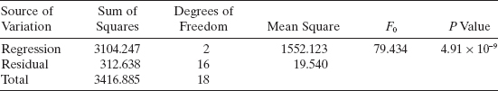
The analysis of variance for this model is shown in Table 7.2. The observed value of F0 = 79.434 and the P value is small, so the hypothesis H0: β1 = β2 = 0 is rejected. We conclude that either the linear or the quadratic term (or both) contribute significantly to the model. The other summary statistics for this model are R2 = 0.9085, se![]() = 0.254, and se
= 0.254, and se![]() = 0.062.
= 0.062.
TABLE 7.1 Hardwood Concentration in Pulp and Tensile Strength of Kraft Paper, Example 7.1
| Hardwood Concentration, xi (%) | Tensile Strength, (psi) y, (psi) |
| 1 | 6.3 |
| 1.5 | 11.1 |
| 2 | 20.0 |
| 3 | 24.0 |
| 4 | 26.1 |
| 4.5 | 30.0 |
| 5 | 33.8 |
| 5.5 | 34.0 |
| 6 | 38.1 |
| 6.5 | 39.9 |
| 7 | 42.0 |
| 8 | 46.1 |
| 9 | 53.1 |
| 10 | 52.0 |
| 11 | 52.5 |
| 12 | 48.0 |
| 13 | 42.8 |
| 14 | 27.8 |
| 15 | 21.9 |

Figure 7.3 Scatterplot of data, Example 7.1.
TABLE 7.2 Analysis of Variance for the Qnadratic Model for Example 7.1
The plot of the residuals versus ŷi is shown in Figure 7.4. This plot does not reveal any serious model inadequacy. The normal probability plot of the residuals, shown in Figure 7.5, is mildly disturbing, indicating that the error distribution has heavier tails than the normal. However, at this point we do not seriously question the normality assumption.
Now suppose that we wish to investigate the contribution of the quadratic term to the model. That is, we wish to test
![]()
We will test these hypotheses using the extra-sum-of-squares method. If β2 = 0, then the reduced model is the straight line y = β0 + β1(x−![]() )+ ε. The least-squares fit is
)+ ε. The least-squares fit is
![]()

Figure 7.4 Plot of residuals ei, versus fitted values ŷi, Example 7.1.

Figure 7.5 Normal probability plot of the residuals, Example 7.1.
The summary statistics for this model are ![]() and SSR (β1|β0) = 1043.427. We note that deleting the quadratic term has substantially affected R2, MSRes, and
and SSR (β1|β0) = 1043.427. We note that deleting the quadratic term has substantially affected R2, MSRes, and ![]() . These summary statistics are much worse than they were for the quadratic model. The extra sum of squares for testing H0:β2 = 0 is
. These summary statistics are much worse than they were for the quadratic model. The extra sum of squares for testing H0:β2 = 0 is
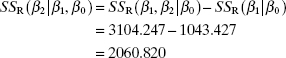
with one degree of freedom. The F statistic is
![]()
and since F0.01,1,16 = 8.53. we conclude that β2 ≠ 0. Thus, the quadratic term contributes significantly to the model.
7.2.2 Piecewise Polynomial Fitting (Splines)
Sometimes we find that a low-order polynomial provides a poor fit to the data, and increasing the order of the polynomial modestly does not substantially improve the situation. Symptoms of this are the failure of the residual sum of squares to stabilize or residual plots that exhibit remaining unexplained structure. This problem may occur when the function behaves differently in different parts of the range of x. Occasionally transformations on x and/or y eliminate this problem. The usual approach, however, is to divide the range of x into segments and fit an appropriate curve in each segment. Spline functions offer a useful way to perform this type of piecewise polynomial fitting.
Splines are piecewise polynomials of order k. The joint points of the pieces are usually called knots. Generally we require the function values and the first k − 1 derivatives to agree at the knots, so that the spline is a continuous function with k − 1 continuous derivatives. The cubic spline (k = 3) is usually adequate for most practical problems.
A cubic spline with h knots, t1 < t2 < … < th, with continuous first and second derivatives can be written as
where
![]()
We assume that the positions of the knots are known. If the knot positions are parameters to be estimated, the resulting problem is a nonlinear regression problem. When the knot positions are known, however, fitting Eq. (7.3) can be accomplished by a straightforward application of linear least squares.
Deciding on the number and position of the knots and the order of the polynomial in each segment is not simple. Wold [1974] suggests that there should be as few knots as possible, with at least four or five data points per segment. Considerable caution should be exercised here because the great flexibility of spline functions makes it very easy to “overfit” the data. Wold also suggests that there should be no more than one extreme point (maximum or minimum) and one point of inflection per segment. Insofar as possible, the extreme points should be centered in the segment and the points of inflection should be near the knots. When prior information about the data-generating process is available, this can sometimes aid in knot positioning.
The basic cubic spline model (7.3) can be easily modified to fit polynomials of different order in each segment and to impose different continuity restrictions at the knots. If all h + 1 polynomial pieces are of order 3, then a cubic spline model with no continuity restrictions is
where (x−t)+0 equals 1 if x > t and 0 if x ≤ t. Thus, if a term βij(x−ti)j+ is in the model, this forces a discontinuity at ti in the jth derivative of S(x). If this term is absent, the jth derivative of S(x) is continuous at ti The fewer continuity restrictions required, the better is the fit because more parameters are in the model, while the more continuity restrictions required, the worse is the fit but the smoother the final curve will be. Determining both the order of the polynomial segments and the continuity restrictions that do not substantially degrade the fit can be done using standard multiple regression hypothesis-testing methods.
As an illustration consider a cubic spline with a single knot at t and no continuity restrictions; for example,
![]()
Note that S(x), S′(x), and S″(x) are not necessarily continuous at t because of the presence of the terms involving β10, β11, and β12 in the model. To determine whether imposing continuity restrictions reduces the quality of the fit, test the hypotheses H0: β10 = 0 [continuity of S(x)], H0: β10 = β11 = 0 [continuity of S(x) and S′(x)], and H0: β10 = β11 = β12 = 0 [continuity of S(x), S′(x), and S″(x)]. To determine whether the cubic spline fits the data better than a single cubic polynomial over the range of x, simply test H0: β10 = β11 = β12 = β13 = 0.
An excellent description of this approach to fitting splines is in Smith [1979]. A potential disadvantage of this method is that the X′X matrix becomes ill-conditioned if there are a large number of knots. This problem can be overcome by using a different representation of the spline called the cubic B-spline. The cubic B-splines are defined in terms of divided differences

and
where γi, i = 1, 2, …, h + 4, are parameters to be estimated. In Eq. (7.5) there are eight additional knots, t−3 < t−2 < t−1 < t0 and th+1 < th+2 < th+3 < th+4. We usually take t0 = xmin and th+1 = xmin; the other knots are arbitrary. For further reading on splines, see Buse and Lim [1977], Curry and Schoenberg [1966], Eubank [1988], Gallant and Fuller [1973], Hayes [1970, 1974], Poirier [1973, 1975], and Wold [1974].
Example 7.2 Voltage Drop Data
The battery voltage drop in a guided missile motor observed over the time of missile flight is shown in Table 7.3. The scatterplot in Figure 7.6 suggests that voltage drop behaves differently in different segments of time, and so we will model the data with a cubic spline using two knots at t1 = 6.5 and t2 = 13 seconds after launch, respectively. This placement of knots roughly agrees with course changes by the missile (with associated changes in power requirements), which are known from trajectory data. The voltage drop model is intended for use in a digital-analog simulation model of the missile.
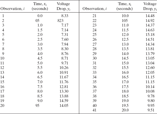

Figure 7.6 Scatterplot of voltage drop data.
The cubic spline model is
![]()
TABLE 7.4 Summary Statistics for the Cubic Spline Model of the Voltage Drop Data


Figure 7.7 Plot of residuals ei, versus fitted values ŷi for the cubic spline model.
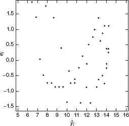
Figure 7.8 Plot of residuals ei, versus fitted values ŷi for the cubic polynomial model.
and the least-squares fit is
![]()
The model summary statistics are displayed in Table 7.4. A plot of the residuals versus ŷi is shown in Figure 7.7. This plot (and other residual plots) does not reveal any serious departures from assumptions, so we conclude that the cubic spline model is an adequate fit to the voltage drop data.
We may easily compare the cubic spline model fit from Example 7.2 with a sample cubic polynomial over the entire time of missile flight; for example,
![]()
This is a simpler model containing fewer parameters and would be preferable to the cubic spline model if it provided a satisfactory fit. The residuals from this cubic polynomial are plotted versus ŷ in Figure 7.8. This plot exhibits strong indication of curvature, and on the basis of this remaining unexplained structure we conclude that the simple cubic polynomial is an inadequate model for the voltage drop data.
We may also investigate whether the cubic spline model improves the fit by testing the hypothesis H0: β1 = β2 = 0 using the extra-sum-of-squares method. The regression sum of squares for the cubic polynomial is
![]()
with three degrees of freedom. The extra sum of squares for testing H0: β1 = β2 = 0 is
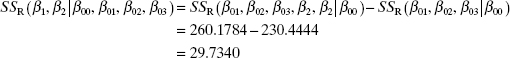
with two degrees of freedom. Since
![]()
which would be referred to the F2, 35 distribution, we reject the hypothesis that H0: β1 = β2 = 0. We conclude that the cubic spline model provides a better fit.
Example 7.3 Piecewise Linear Regression
An important special case of practical interest involves fitting piecewise linear regression models. This can be treated easily using linear splines. For example, suppose that there is a single knot at t and that there could be both a slope change and a discontinuity at the knot. The resulting linear spline model is
![]()
Now if x ≤ t, the straight-line model is
![]()
and if x > t, the model is
![]()
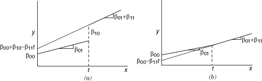
Figure 7.9 Piecewise linear regression: (a) discontinuity at the knot; (b) continuous piecewise linear regression model
That is, if x ≤ t, the model has intercept β00 and slope β01, while if x > t, the intercept is β00 + β10 − β11t and the slope is β01 + β11. The regression function is shown in Figure 7.9a. Note that the parameter β10 represents the difference in mean response at the knot t.
A smoother function would result if we required the regression function to be continuous at the knot. This is easily accomplished by deleting the term β10(x−t)0+ from the original model, giving
![]()
Now if x ≤ t, the model is
![]()
and if x > t, the model is
![]()
The two regression functions are shown in Figure 7.9b.
7.2.3 Polynomial and Trigonometric Terms
It is sometimes useful to consider models that combine both polynomial and trigonometric terms as alternatives to models that contain polynomial terms only. In particular, if the scatter diagram indicates that there may be some periodicity or cyclic behavior in the data, adding trigonometric terms to the model may be very beneficial, in that a model with fewer terms may result than if only polynomial terms were employed. This benefit has been noted by both Graybill [1976] and Eubank and Speckman [1990].
The model for a single regressor x is
![]()
If the regressor x is equally spaced, then the pairs of terms sin(jx) and cos(jx) are orthogonal. Even without exactly equal spacing, the correlation between these terms will usually be quite small.
Eubank and Speckman [1990] use the voltage drop data of Example 7.2 to illustrate fitting a polynomial-trigonometric regression model. They first rescale the regressor x (time) so that all of the observations are in the interval (0, 2π) and fit the model above with d = 2 and r = 1 so that the model is quadratic in time and has a pair of sine-cosine terms. Thus, their model has only four terms, whereas our spline regression model had five. Eubank and Speckman obtain R2 = 0.9895 and MSRes = 0.0767, results that are very similar to those found for the spline model (refer to Table 7.4). Since the voltage drop data exhibited some indication of periodicity in the scatterplot (Figure 7.6), the polynomial-trigonometric regression model is certainly a good alternative to the spline model. It has one fewer term (always a desirable property) but a slightly larger residual mean square. Working with a rescaled version of the regressor variable might also be considered a potential disadvantage by some users.
7.3 NONPARAMETRIC REGRESSION
Closely related to piecewise polynomial regression is nonparametric regression. The basic idea of nonparametric regression is to develop a model-free basis for predicting the response over the range of the data. The early approaches to nonparametric regression borrow heavily from nonparametric density estimation. Most of the nonparametric regression literature focuses on a single regressor; however, many of the basic ideas extend to more than one.
A fundamental insight to nonparametric regression is the nature of the predicted value. Consider standard ordinary least squares. Recall

As a result,
![]()
In other words, the predicted value for the ith response is simply a linear combination of the original data.
7.3.1 Kernel Regression
One of the first alternative nonparametric approaches is the kernel smoother, which uses a weighted average of the data. Let ![]() be the kernel smoother estimate of the ith response. For a kernel smoother,
be the kernel smoother estimate of the ith response. For a kernel smoother,
![]()
where Σnj=1 wij = 1. As a result,
![]()
where S = [wij] is the “smoothing” matrix. Typically, the weights are chosen such that wij ≅ 0 for all yi's outside of a defined “neighborhood” of the specific location of interest. These kernel smoothers use a bandwidth, b, to define this neighborhood of interest. A large value for b results in more of the data being used to predict the response at the specific location. Consequently, the resulting plot of predicted values becomes much smoother as b increases. Conversely, as b decreases, less of the data are used to generate the prediction, and the resulting plot looks more “wiggly” or bumpy.
This approach is called a kernel smoother because it uses a kernel function, K, to specify the weights. Typically, these kernel functions have the following properties:
- K(t) ≥ 0 for all t

- K(−t) = K(t) (symmetry)
These are also the properties of a symmetric probability density function, which emphasizes the relationship back to nonparametric density estimation. The specific weights for the kernel smoother are given by

Table 7.5 summarizes the kernels used in S-PLUS. The properties of the kernel smoother depend much more on the choice of the bandwidth than the actual kernel function.
7.3.2 Locally Weighted Regression (Loess)
Another nonparametric alternative is locally weighted regression, often called loess. Like kernel regression, loess uses the data from a neighborhood around the specific location. Typically, the neighborhood is defined as the span, which is the fraction of the total points used to form neighborhoods. A span of 0.5 indicates that the closest half of the total data points is used as the neighborhood. The loess procedure then uses the points in the neighborhood to generate a weighted least-squares estimate of the specific response. The weighted least-squares procedure uses a low-order polynomial, usually simple linear regression or a quadratic regression model. The weights for the weighted least-squares portion of the estimation are based on the distance of the points used in the estimation from the specific location of interest. Most software packages use the tri-cube weighting function as its default. Let x0 be the specific location of interest, and let Δ(x0) be the distance the farthest point in the neighborhood lies from the specific location of interest. The tri-cube weight function is
TABLE 7.5 Snmmary of the Kernel Functions Used in S-PLUS
| Box | |
| Triangle |  |
| Parzen |  |
| Normal |
![]()
where
![]()
We can summarize the loess estimation procedure by
![]()
where S is the smoothing matrix created by the locally weighted regression.
The concept of sum of squared residuals carries over to nonparametric regression directly. In particular,

Asymptotically, these smoothing procedures are unbiased. As a result, the asymptotic expected value for SSRes is

It is important to note that S is a square n × n matrix. As a result, trace[S′] = trace[S]; thus,
![]()
In some sense, [2 trace(S) − trace(S′S)] represents the degrees of freedom associated with the total model. In some packages, [2 trace(S) − trace(S′S)] is called the equivalent number of parameters and represents a measure of the complexity of the estimation procedure. A common estimate of σ2 is

Finally, we can define a version of R2 by
![]()
whose interpretation is the same as before in ordinary least squares. All of this extends naturally to the multiple regression case, and S-PLUS has this capability.
Example 7.4 Applying Loess Regression to the Windmill Data
In Example 5.2, we discussed the data collected by an engineer who investigated the relationship of wind velocity and the DC electrical output for a windmill. Table 5.5 summarized these data. Ultimately in this example, we developed a simple linear regression model involving the inverse of the wind velocity. This model provided a nice basis for modeling the fact that there is a true upper bound to the DC output the windmill can generate.
An alternative approach to this example uses loess regression. The appropriate SAS code to analyze the windmill data is:

Figure 7.10 The loess fit to the windmill data.

Figure 7.11 The residuals versus fitted values for the loess fit to the windmill data.
TABLE 7.6 SAS Output for Loess Fit to Windmill Data

proc loess;
model output = velocity / degree = 2 dfmethod = exact
residual;
Figure 7.10 gives the loess fit to the data using SAS's default settings, and Table 7.6 summarizes the resulting SAS report. Figure 7.11, which gives the residuals versus fitted values, shows no real problems. Figure 7.12 gives the normal probability plot, which, although not perfect, does not indicate any serious problems.

Figure 7.12 The normal probability plot of the residuals for the loess fit to the windmill data.
The loess fit to the data is quite good and compares favorably with the fit we generated earlier using ordinary least squares and the inverse of the wind velocity.
The report indicates an R2 of 0.98, which is the same as our final simple linear regression model. Although the two R2 values are not directly comparable, they both indicate a very good fit. The loess MSRes is 0.1017, compared to a value of 0.0089 for the simple linear regression model. Clearly, both models are competitive with one another. Interestingly, the loess fit requires an equivalent number of parameters of 4.4, which is somewhere between a cubic and quartic model. On the other hand, the simple linear model using the inverse of the wind velocity requires only two parameters; hence, it is a much simpler model. Ultimately, we prefer the simple linear regression model since it is simpler and corresponds to known engineering theory. The loess model, on the other hand, is more complex and somewhat of a “black box”.
The R code to perform the analysis of these data is:
windmill < - read.table(<windmill_loess.txt=, header = TRUE,
sep = < =) wind.model < - loess(output ~ velocity,
data = windmill)
summary(wind.model)
yhat < - predict(wind.model)
plot(windmill$velocity,yhat)
7.3.3 Final Cautions
Parametric and nonparametric regression analyses each have their advantages and disadvantages. Often, parametric models are guided by appropriate subject area theory. Nonparametric models almost always reflect pure empiricism.
One should always prefer a simple parametric model when it provides a reasonable and satisfactory fit to the data. The complexity issue is not trivial. Simple models provide an easy and convenient basis for prediction. In addition, the model terms often have important interpretations. There are situations, like the windmill data, where transformations of either the response or the regressor are required to provide an appropriate fit to the data. Again, one should prefer the parametric model, especially when subject area theory supports the transformation used.
On the other hand, there are many situations where no simple parametric model yields an adequate or satisfactory fit to the data, where there is little or no subject area theory to guide the analyst, and where no simple transformation appears appropriate. In such cases, nonparametric regression makes a great deal of sense. One is willing to accept the relative complexity and the black-box nature of the estimation in order to give an adequate fit to the data.
7.4 POLYNOMIAL MODELS IN TWO OR MORE VARIABLES
Fitting a polynomial regression model in two or more regressor variables is a straightforward extension of the approach in Section 7.2.1. For example, a second-order polynomial model in two variables would be
Note that this model contains two linear effect parameters β1 and β2 two quadratic effect parameters β11 and β21 and an interaction effect parameter β12.
Fitting a second-order model such as Eq. (7.7) has received considerable attention, both from researchers and from practitioners. We usually call the regression function
![]()
a response surface. We may represent the two-dimensional response surface graphically by drawing the x1 and x2 axes in the plane of the paper and visualizing the E(y) axis perpendicular to the plane of the paper. Plotting contours of constant expected response E(y) produces the response surface. For example, refer to Figure 3.3, which shows the response surface
![]()
Note that this response surface is a hill, containing a point of maximum response. Other possibilities include a valley containing a point of minimum response and a saddle system. Response surface methodology (RSM) is widely applied in industry for modeling the output response(s) of a process in terms of the important controllable variables and then finding the operating conditions that optimize the response. For a detailed treatment of response surface methods see Box and Draper [1987], Box, Hunter, and Hunter [1978], Khuri and Cornell [1996], Montgomery [2009], and Myers, Montgomery and Anderson Cook [2009].
We now illustrate fitting a second-order response surface in two variables. Panel A of Table 7.7 presents data from an experiment that was performed to study the effect of two variables, reaction temperature (T) and reactant concentration (C), on the percent conversion of a chemical process (y). The process engineers had used an approach to improving this process based on designed experiments. The first experiment was a screening experiment involving several factors that isolated temperature and concentration as the two most important variables. Because the experimenters thought that the process was operating in the vicinity of the optimum, they elected to fit a quadratic model relating yield to temperature and concentration.
Panel A of Table 7.7 shows the levels used for T and C in the natural units of measurements. Panel B shows the levels in terms of coded variables x1 and x2.
Figure 7.13 shows the experimental design in Table 7.5 graphically. This design is called a central composite design, and it is widely used for fitting a second-order response surface. Notice that the design consists of four runs at the comers of a square plus four runs at the center of this square plus four axial runs, In terms of the coded variables the comers of the square are (x1, x2) = (−1, −1), (1, −1), (−1, −1), (1, 1); the center points are at (x1, x2) = (0, 0); and the axial runs are at (x1, x2) = (−1.414, 0), (1.414, 0), (0, −1.414), (0, 1.414).
TABLE 7.7 Central Composite Design for Chemical Process Example


Figure 7.13 Central composite design for the chemical process example.
We fit the second-order model
![]()
using the coded variables, as that is the standard practice in RSM work. The X matrix and y vector for this model are

Notice that we have shown the variables associated with each column above that column in the X matrix. The entries in the columns associated with x21 and x22 are found by squaring the entries in columns x1 and x2, respectively, and the entries in the x1x2 column are found by multiplying each entry from x1 by the corresponding entry from x2. The X′X matrix and X′y vector are
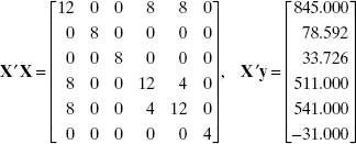
and from ![]() we obtain
we obtain
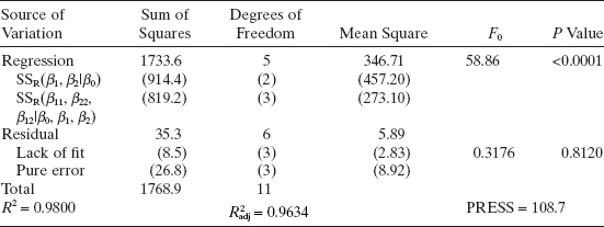
TABLE 7.8 Analysis of Variance for the Chemical Process Example

Therefore, the fitted model for percent conversion is
![]()
In terms of the natural variables, the model is
![]()
Table 7.8 shows the analysis of variance for this model. Because the experimental design has four replicate runs, the residual sum of squares can be partitioned into pure-error and lack-of-fit components. The lack-of-fit test in Table 7.8 is testing the lack of fit for the quadratic model. The P value for this test is large (P = 0.8120), implying that the quadratic model is adequate. Therefore, the residual mean square with six degrees of freedom is used for the remaining analysis. The F test for significance of regression is F0 = 58.86; and because the P value is very small, we would reject the hypothesis H0: β1 = β2 = β11 = β22 = β12 = 0, concluding that at least some of these parameters are nonzero. This table also shows the sum of squares for testing the contribution of only the linear terms to the model [SSR(β1, β2|β0) = 918.4 with two degrees of freedom] and the sum of squares for testing the contribution of the quadratic terms given that the model already contains the linear terms [SSR(β11, β22, β12|β0, β1, β2) = 819.2 with three degrees of freedom]. Comparing both of the corresponding mean squares to the residual mean square gives the following F statistics
TABLE 7.9 Tests on the Individual Variables, Chemical Process Quadratic Model

![]()
for which P = 5.2 × 10—5 and
![]()
for which P = 0.0002. Therefore, both the linear and quadratic terms contribute significantly to the model.
Table 7.9 shows t tests on each individual variable. All t values are large enough for us to conclude that there are no nonsignificant terms in the model. If some of these t statistics had been small, some analysts would drop the nonsignificant variables for the model, resulting in a reduced quadratic model for the process. Generally, we prefer to fit the full quadratic model whenever possible, unless there are large differences between the full and reduced model in terms of PRESS and adjusted R2. Table 7.8 indicates that the R2 and adjusted R2 values for this model are satisfactory. R2prediction, based on PRESS, is
![]()
indicating that the model will probably explain a high percentage (about 94%) of the variability in new data.
Table 7.10 contains the observed and predicted values of percent conversion, the residuals, and other diagnostic statistics for this model. None of the studentized residuals or the values of R-student are large enough to indicate any potential problem with outliers. Notice that the hat diagonals hii take on only two values, either 0.625 or 0.250. The values of hii = 0.625 are associated with the four runs at the corners of the square in the design and the four axial runs. All eight of these points are equidistant from the center of the design; this is why all of the hii values are identical. The four center points all have hii = 0.250. Figures 7.14, 7.15, and 7.16 show a normal probability plot of the studentized residuals, a plot of the studentized residuals versus the predicted values ŷi, and a plot of the studentized residuals versus run order. None of these plots reveal any model inadequacy.
TABLE 7.10 Observed Values, Predicted Values, Residuals, and Other Diagnostics for the Cbemical Process Example

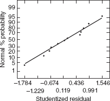
Figure 7.14 Normal probability plot of the studentized residuals, chemical process example.

Figure 7.15 Plot of studentized versus predicted conversion, chemical process example.

Figure 7.16 Plot of the studentized residuals run order, chemical process example.

Figure 7.17 (a) Response surface of predicted conversion. (b) Contour plot of predicted conversion.
Plots of the conversion response surface and the contour plot, respectively, for the fitted model are shown in panels a and b of Figure 7.17. The response surface plots indicate that the maximum percent conversion occurs at about 245°C and 20% concentration.
In many response surface problems the experimenter is interested in predicting the response y or estimating the mean response at a particular point in the process variable space. The response surface plots in Figure 7.17 give a graphical display of these quantities. Typically, the variance of the prediction is also of interest, because this is a direct measure of the likely error associated with the point estimate produced by the model. Recall that the variance of the estimate of the mean response at the point x0 is given by Var[ŷ(x0)] = σ2x′0(X′X)−1x0. Plots of ![]() , with σ2 estimated by the residual mean square MSRes = 5.89 for this model for all values of x0 in the region of experimentation, are presented in panels a and b of Figure 7.18. Both the response surface in Figure 7.18a and the contour plot of constant
, with σ2 estimated by the residual mean square MSRes = 5.89 for this model for all values of x0 in the region of experimentation, are presented in panels a and b of Figure 7.18. Both the response surface in Figure 7.18a and the contour plot of constant ![]() in Figure 7.18b show that the
in Figure 7.18b show that the ![]() is the same for all points x0 that are the same distance from the center of the design. This is a result of the spacing of the axial runs in the central composite design at 1.414 units from the origin (in the coded variables) and is a design property called rotatability. This is a very important property for a second-order response surface design and is discussed in detail in the references given on RSM.
is the same for all points x0 that are the same distance from the center of the design. This is a result of the spacing of the axial runs in the central composite design at 1.414 units from the origin (in the coded variables) and is a design property called rotatability. This is a very important property for a second-order response surface design and is discussed in detail in the references given on RSM.
7.5 ORTHOGONAL POLYNOMIALS
We have noted that in fitting polynomial models in one variable, even if nonessential ill-conditioning is removed by centering, we may still have high levels of multicollinearity. Some of these difficulties can be eliminated by using orthogonal polynomials to fit the model.

Figure 7.18 (a) Response surface plot of ![]() . (b) Contour plot of
. (b) Contour plot of ![]() .
.
Suppose that the model is
Generally the columns of the X matrix will not be orthogonal. Furthermore, if we increase the order of the polynomial by adding a term βk+1xk+1, we must recompute (X′X)−1 and the estimates of the lower order parameters ![]() will change.
will change.
Now suppose that we fit the model
where Pu(xi) is a uth-order orthogonal polynomial defined such that

Then the model becomes y = Xα + ε, where the X matrix is

Since this matrix has orthogonal columns, the X′X matrix is
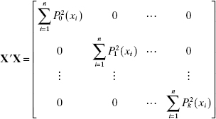
The least-squares estimators of α are found from (X′X)−1X′y as

Since P0(xi) is a polynomial of degree zero, we can set P0(xi) = 1, and consequently
![]()
The residual sum of squares is
The regression sum of squares for any model parameter does not depend on the other parameters in the model. This regression sum of squares is
If we wish to assess the significance of the highest order term, we should test H0: αk = 0 [this is equivalent to testing H0: βk = 0 in Eq. (7.4)]; we would use

as the F statistic. Furthermore, note that if the order of the model is changed to k + r, ouly the r new coefficients must be computed. The coefficients ![]() do not change due to the orthogonality property of the polynomials. Thus, sequential fitting of the model is computationally easy.
do not change due to the orthogonality property of the polynomials. Thus, sequential fitting of the model is computationally easy.
The orthogonal polynomials Pj(xi) are easily constructed for the case where the levels of x are equally spaced. The first five orthogonal polynomials are

where d is the spacing between the levels of x and the {λj} are constants chosen so that the polynomials will have integer values. A brief table of the numerical values of these orthogonal polynomials is given in Table A.5. More extensive tables are found in DeLury [1960] and Pearson and Hartley [1966]. Orthogonal polynomials can also be constructed and used in cases where the x's are not equally spaced. A survey of methods for generating orthogonal polynomials is in Seber [1977, Ch. 8].
Example 7.5 Orthogonal Polynomials
An operations research analyst has developed a computer simulation model of a single item inventory system. He has experimented with the simulation model to investigate the effect of various reorder quantities on the average annual cost of the inventory. The data are shown in Table 7.11.
TABLE 7.11 Inventory Simnlatian Ontpnt far Example 7.5
| Reorder Quantity, xi | Average Annual Cost, yi |
| 50 | $335 |
| 75 | 326 |
| 100 | 316 |
| 125 | 313 |
| 150 | 311 |
| 175 | 314 |
| 200 | 318 |
| 225 | 328 |
| 250 | 337 |
| 275 | 345 |
TABLE 7.12 Coefficients of Orthogonal Polynomials for Example 7.5

Since we know that average annual inventory cost is a convex function of the reorder quantity, we suspect that a second-order polynomial is the highest order model that must be considered. Therefore, we will fit
![]()
The coefficients of the orthogonal polynomials P0(xi), P1(xi), and P2(xi), obtained from Table A.5, are shown in Table 7.12.
Thus,

TABLE 7.13 Analysis of Variance for the Quadratic Model in Example 7.5

and

The fitted model is
![]()
The regression sum of squares is

The analysis of variance is shown in Table 7.13. Both the linear and quadratic terms contribute significantly to the model. Since these terms account for most of the variation in the data, we tentatively adopt the quadratic model subject to a satisfactory residual analysis.
We may obtain a fitted equation in terms of the original regressor by substituting for Pj(xi) as follows:
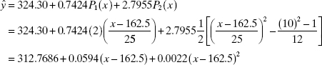
This form of the model should be reported to the user.
PROBLEMS
7.1 Consider the values of x shown below:
![]()
Suppose that we wish to fit a second-order model using these levels for the regressor variable x. Calculate the correlation between x and x2. Do you see any potential difficulties in fitting the model?
7.2 A solid-fuel rocket propellant loses weight after it is produced. The following data are available:
| Months since Production, x | Weight Loss, y (kg) |
| 0.25 | 1.42 |
| 0.50 | 1.39 |
| 0.75 | 1.55 |
| 1.00 | 1.89 |
| 1.25 | 2.43 |
| 1.50 | 3.15 |
| 1.75 | 4.05 |
| 2.00 | 5.15 |
| 2.25 | 6.43 |
| 2.50 | 7.89 |
- Fit a second-order polynomial that expresses weight loss as a function of the number of months since production.
- Test for significance of regression.
- Test the hypothesis H0: β2 = 0. Comment on the need for the quadratic term in this model.
- Are there any potential hazards in extrapolating with this model?
7.3 Refer to Problem 7.2. Compute the residuals for the second-order model. Analyze the residuals and comment on the adequacy of the model.
7.4 Consider the data shown below:

- Fit a second-order polynomial model to these data.
- Test for significance of regression.
- Test for lack of fit and comment on the adequacy of the second-order model.
- Test the hypothesis H0: β2 = 0. Can the quadratic term be deleted from this equation?
7.5 Refer to Problem 7.4. Compute the residuals from the second-order model. Analyze the residuals and draw conclusions about the adequacy of the model.
7.6 The carbonation level of a soft drink beverage is affected by the temperature of the product and the filler operating pressure. Twelve observations were obtained and the resulting data are shown below.

- Fit a second-order polynomial.
- Test for significance of regression.
- Test for lack of fit and draw conclusions.
- Does the interaction term contribute significantly to the model?
- Do the second-order terms contribute significantly to the model?
7.7 Refer to Problem 7.6. Compute the residuals from the second-order model. Analyze the residuals and comment on the adequacy of the model.
7.8 Consider the data in Problem 7.2.
- Fit a second-order model to these data using orthogonal polynomials.
- Suppose that we wish to investigate the addition of a third-order term to this model. Comment on the necessity of this additional term. Support your conclusions with an appropriate statistical analysis.
7.9 Suppose we wish to fit the piecewise quadratic polynomial with a knot at x = t:
![]()
- Show how to test the hypothesis that this quadratic spline model fits the data significantly better than an ordinary quadratic polynomial.
- The quadratic spline polynomial model is not continuous at the knot t. How can the model be modified so that continuity at x = t is obtained?
- Show how the model can be modified so that both E(y) and dE(y)/dx are continuous at x = t.
- Discuss the significance of the continuity restrictions on the model in parts b and c. In practice, how would you select the type of continuity restrictions to impose?
7.10 Consider the delivery time data in Example 3.1. Is there any indication that a complete second-order model in the two regressions cases and distance is preferable to the first-order model in Example 3.1?
7.11 Consider the patient satisfaction data in Section 3.6. Fit a complete second-order model to those data. Is there any indication that adding these terms to the model is necessary?
7.12 Suppose that we wish to fit a piecewise polynomial model with three segments: if x < t1, the polynomial is linear; if t1 ≤ x < t2, the polynomial is quadratic; and if x > t2, the polynomial is linear. Consider the model
![]()
- Does this segmented polynomial satisfy our requirements If not, show how it can be modified to do so.
- Show how the segmented model would be modified to ensure that E(y) is continuous at the knots t1 and t2.
- Show how the segmented model would be modified to ensure that both E(y) and dE(y)/dx are continuous at the knots t1 and t2.
7.13 An operations research analyst is investigating the relationship between production lot size x and the average production cost per unit y. A study of recent operations provides the following data:
![]()
The analyst suspects that a piecewise linear regression model should be fit to these data. Estimate the parameters in such a model assuming that the slope of the line changes at x = 200 units. Do the data support the use of this model?
7.14 Modify the model in Problem 7.13 to investigate the possibility that a discontinuity exists in the regression function at x = 200 units. Estimate the parameters in this model. Test appropriate hypotheses to determine if the regression function has a change in both the slope and the intercept at x = 200 units.
7.15 Consider the polynomial model in Problem 7.13. Find the variance inflation factors and comment on multicollinearity in this model.
7.16 Consider the data in Problem 7.2.
- Fit a second-order model y = β0 + β1x + β11x2 + ε to the data. Evaluate the variance inflation factors.
- Fit a second-order model y = β0 + β1(x−) + β11(x−) + ε to the data. Evaluate the variance inflation factors.
- What can you conclude about the impact of centering the x's in a polynomial model on multicollinearity?
7.17 Chemical and mechanical engineers often need to know the vapor pressure of water at various temperatures (the “infamous” steam tables can be used for this). Below are data on the vapor pressure of water (y) at various temperatures.
| Vapor Pressure, y (mmHg) | Temperature, x (°C) |
| 9.2 | 10 |
| 17.5 | 20 |
| 31.8 | 30 |
| 55.3 | 40 |
| 92.5 | 50 |
| 149.4 | 60 |
- Fit a first-order model to the data. Overlay the fitted model on the scatterplot of y versus x. Comment on the apparent fit of the model.
- Prepare a scatterplot of predicted y versus the observed y. What does this suggest about model fit?
- Plot residuals versus the fitted or predicted y. Comment on model adequacy.
- Fit a second-order model to the data. Is there evidence that the quadratic term is statistically significant?
- Repeat parts a–c using the second-order model. Is there evidence that the second-order model provides a better fit to the vapor pressure data?
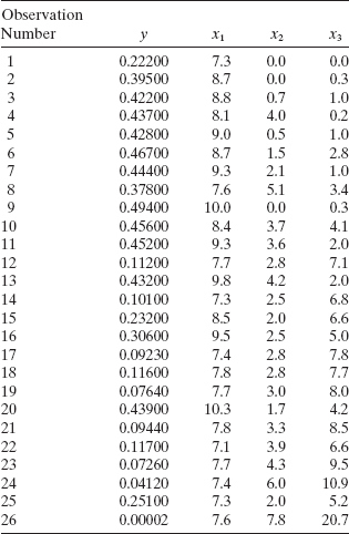
7.18 An article in the Journal of Pharmaceutical Sciences (80, 971–977, 1991) presents data on the observed mole fraction solubility of a solute at a constant temperature, along with x1 = dispersion partial solubility, x2 = dipolar partial solubility, and x3 = hydrogen bonding Hansen partial solubility. The response y is the negative logarithm of the mole fraction solubility.
- Fit a complete quadratic model to the data.
- Test for significance of regression, and construct t statistics for each model parameter. Interpret these results.
- Plot residuals and comment on model adequacy.
- Use the extra-sum-of-squares method to test the contribution of all second-order terms to the model.
7.19 Consider the quadratic regression model from Problem 7.18. Find the variance inflation factors and comment on multicollinearity in this model.
7.20 Consider the solubility data from Problem 7.18. Suppose that a point of interest is x1 = 8.0, x2 = 3.0, and x3 = 5.0.
- For the quadratic model from Problem 7.18, predict the response at the point of interest and find a 95% confidence interval on the mean response at that point.
- Fit a model that includes only the main effects and two-factor interactions to the solubility data. Use this model to predict the response at the point of interest. Find a 95% confidence interval on the mean response at that point.
- Compare the lengths of the confidence intervals in parts a and b. Can you draw any conclusions about the best model from this comparison?
7.21 Below are data on y = green liquor (g/l) and x = paper machine speed (ft/min) from a kraft paper machine. (The data were read from a graph in an article in the Tappi Journal, March 1986.)
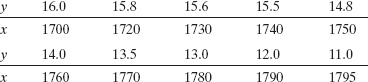
- Fit the model y = β0 + β1x + β2x2 + ε to the data.
- Test for significance of regression using = 0.05. What are your conclusions?
- Test the contribution of the quadratic term to the model, the contribution of the linear term, using an F statistic. If α = 0.05, what conclusion can you draw?
- Plot the residuals from the model. Does the model fit seem satisfactory?
7.22 Reconsider the data from Problem 7.21. Suppose that it is important to predict the response at the points x = 1750 and x = 1775.
- Find the predicted response at these points and the 95% prediction intervals for the future observed response at these points.
- Suppose that a first-order model is also being considered. Fit this model and find the predicted response at these points. Calculate the 95% prediction intervals for the future observed response at these points. Does this give any insight about which model should be preferred?