
CHAPTER 5
TRANSFORMATIONS AND WEIGHTING TO CORRECT MODEL INADEQUACIES
5.1 INTRODUCTION
Chapter 4 presented several techniques for checking the adequacy of the linear regression model. Recall that regression model fitting has several implicit assumptions, including the following:
- The model errors have mean zero and constant variance and are uncorrelated.
- The model errors have a normal distribution—this assumption is made in order to conduct hypothesis tests and construct CIs—under this assumption, the errors are independent.
- The form of the model, including the specification of the regressors, is correct.
Plots of residuals are very powerful methods for detecting violations of these basic regression assumptions. This form of model adequacy checking should be conducted for every regression model that is under serious consideration for use in practice.
In this chapter, we focus on methods and procedures for building regression models when some of the above assumptions are violated. We place considerable emphasis on data transformation. It is not unusual to find that when the response and/or the regressor variables are expressed in the correct scale of measurement or metric, certain violations of assumptions, such as inequality of variance, are no longer present. Ideally, the choice of metric should be made by the engineer or scientist with subject-matter knowledge, but there are many situations where this information is not available. In these cases, a data transformation may be chosen heuristically or by some analytical procedure.
The method of weighted least squares is also useful in building regression models in situations where some of the underlying assumptions are violated. We will illustrate how weighted least squares can be used when the equal-variance assumption is not appropriate. This technique will also prove essential in subsequent chapters when we consider other methods for handling nonnormal response variables.
5.2 VARIANCE-STABILIZING TRANSFORMATIONS
The assumption of constant variance is a basic requirement of regression analysis. A common reason for the violation of this assumption is for the response variable y to follow a probability distribution in which the variance is functionally related to the mean. For example, if y is a Poisson random variable in a simple linear regression model, then the variance of y is equal to the mean. Since the mean of y is related to the regressor variable x, the variance of y will be proportional to x. Variance-stabilizing transformations are often useful in these cases. Thus, if the distribution of y is Poisson, we could regress ![]() against x since the variance of the square root of a Poisson random variable is independent of the mean. As another example, if the response variable is a proportion (0 ≤ yi ≤ 1) and the plot of the residuals versus ŷi has the double-bow pattern of Figure 4.5c, the arcsin transformation
against x since the variance of the square root of a Poisson random variable is independent of the mean. As another example, if the response variable is a proportion (0 ≤ yi ≤ 1) and the plot of the residuals versus ŷi has the double-bow pattern of Figure 4.5c, the arcsin transformation ![]() is appropriate.
is appropriate.
Several commonly used variance-stabilizing transformations are summarized in Table 5.1. The strength of a transformation depends on the amount of curvature that it induces. The transformations given in Table 5.1 range from the relatively mild square root to the relatively strong reciprocal. Generally speaking, a mild transformation applied over a relatively narrow range of values (e.g., ymax/ymin < 2, 3) has little effect. On the other hand, a strong transformation over a wide range of values will have a dramatic effect on the analysis.
Sometimes we can use prior experience or theoretical considerations to guide us in selecting an appropriate transformation. However, in many cases we have no a priori reason to suspect that the error variance is not constant. Our first indication of the problem is from inspection of scatter diagrams or residual analysis. In these cases the appropriate transformation may be selected empirically.
TABLE 5.1 Useful Variance-Stabilizing Transformations
| Relationship of σ2 to E(y) | Transfonnation |
| σ2 ∝ constant | y′ = y (no transformation) |
| σ2 ∝ E(y) | |
| σ2 ∝ E(y)[1 – E(y] | |
| σ2 ∝ [E(y)]2 | y′ = In(y)(log) |
| σ2 ∝ [E(y)]3 | y′ = y−1/2 (reciprocal square root) |
| σ2 ∝ [E(y)]4 | y′ = y−1(reciprocal) |
It is important to detect and correct a nonconstant error variance. If this problem is not eliminated, the least-squares estimators will still be unbiased, but they will no longer have the minimum-variance property. This means that the regression coefficients will have larger standard errors than necessary. The effect of the transformation is usually to give more precise estimates of the model parameters and increased sensitivity for the statistical tests.
When the response variable has been reexpressed, the predicted values are in the transformed scale. It is often necessary to convert the predicted values back to the original units. Unfortunately, applying the inverse transformation directly to the predicted values gives an estimate of the median of the distribution of the response instead of the mean. It is usually possible to devise a method for obtaining unbiased predictions in the original units. Procedures for producing unbiased point estimates for several standard transformations are given by Neyman and Scott [1960]. Miller [1984] also suggests some simple solutions to this problem. Confidence or prediction intervals may be directly converted from one metric to another, as these interval estimates are percentiles of a distribution and percentiles are unaffected by transformation. However, there is no assurance that the resulting intervals in the original units are the shortest possible intervals. For further discussion, see Land [1974].
Example 5.1 The Electric Utility Data
An electric utility is interested in developing a model relating peak-hour demand (y) to total energy usage during the month (x). This is an important planning problem because while most customers pay directly for energy usage (in kilowatt-hours), the generation system must be large enough to meet the maximum demand imposed. Data for 53 residential customers for the month of August are shown in Table 5.2, and a scatter diagram is given in Figure 5.1. As a starting point, a simple linear regression model is assumed, and the least-squares fit is
![]()
The analysis of variance is shown in Table 5.3. For this model R2 = 0.7046; that is, about 70% of the variability in demand is accounted for by the straight-line fit to energy usage. The summary statistics do not reveal any obvious problems with this model.
A plot of the R-student residuals versus the fitted values ŷi is shown in Figure 5.2. The residuals form an outward-opening funnel, indicating that the error variance is increasing as energy consumption increases. A transformation may be helpful in correcting this model inadequacy. To select the form of the transformation, note that the response variable y may be viewed as a “count” of the number of kilowatts used by a customer during a particular hour. The simplest probabilistic model for count data is the Poisson distribution. This suggests regressing y* = ![]() on x as a variancestabilizing transformation. The resulting least-squares fit is
on x as a variancestabilizing transformation. The resulting least-squares fit is
![]()
The R-student values from this least-squares fit are plotted against ŷ*i in Figure 5.3. The impression from examining this plot is that the variance is stable; consequently, we conclude that the transformed model is adequate. Note that there is one suspiciously large residual (customer 26) and one customer whose energy usage is somewhat large (customer 50). The effect of these two points on the fit should be studied further before the model is released for use.
TABLE 5.2 Demand (y) and Energy Usage (x) Data for 53 Residential Cnstomers, August
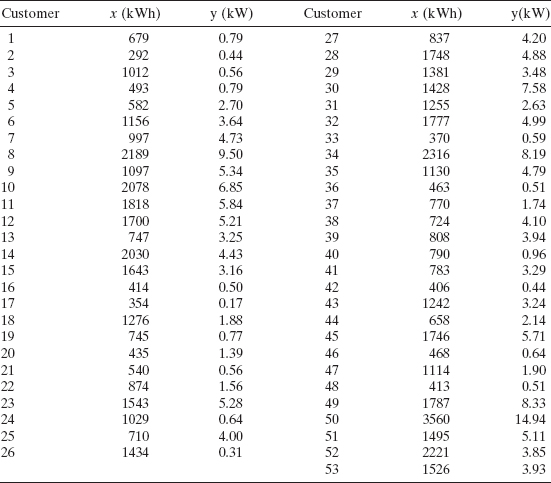

Figure 5.1 Scatter diagram of the energy demand (kW) versus energy usage (kWh), Example 5.1.
TABLE 5.3 Analysis of Variance for Regression of y on x for Example 5.1
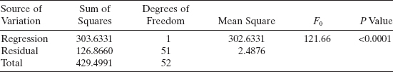
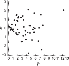
Figure 5.2 Plot of R-student values ti versus fitted values ŷi, Example 5.1.
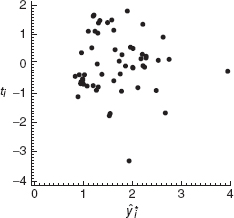
Figure 5.3 Plot of R-student values ti versus fitted values ŷ*i for the transformed data, Example 5.1.
5.3 TRANSFORMATIONS TO LINEARIZE THE MODEL
The assumption of a linear relationship between y and the regressors is the usual starting point in regression analysis. Occasionally we find that this assumption is inappropriate. Nonlinearity may be detected via the lack-of-fit test described in Section 4.5 or from scatter diagrams, the matrix of scatterplots, or residual plots such as the partial regression plot. Sometimes prior experience or theoretical considerations may indicate that the relationship between y and the regressors is not linear. In some cases a nonlinear function can be linearized by using a suitable transformation. Such nonlinear models are called intrinsically or transformably linear.
Several linearizable functions are shown in Figure 5.4. The corresponding nonlinear functions, transformations, and resulting linear forms are shown in Table 5.4. When the scatter diagram of y against x indicates curvature, we may be able to match the observed behavior of the plot to one of the curves in Figure 5.4 and use the linearized form of the function to represent the data.
To illustrate a nonlinear model that is intrinsically linear, consider the exponential function
![]()
This function is intrinsically linear since it can be transformed to a straight line by a logarithmic transformation
![]()
or
![]()
as shown in Table 5.4. This transformation requires that the transformed error terms ε′ = ln ε are normally and independently distributed with mean zero and variance σ2. This implies that the multiplicative error ε in the original model is log normally distributed. We should look at the residuals from the transformed model to see if the assumptions are valid. Generally if x and/or y are in the proper metric, the usual least-squares assumptions are more likely to be satisfied, although it is no unusual to discover at this stage that a nonlinear model is preferable (see Chapter 12).
Various types of reciprocal transformations are also useful. For example, the model
![]()
can be linearized by using the reciprocal transformation x′ = 1/x. The resulting linearized model is
![]()
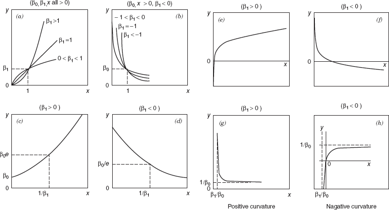
Figure 5.4 Linearizable functions. (From Daniel and Wood [1980], used with permission of the publisher.)
TABLE 5.4 Linearizable Functions and Corresponding Linear Form
Other models that can be linearized by reciprocal transformations are
![]()
and
![]()
This last model is illustrated in Figures 5.4g, h.
When transformations such as those described above are employed, the least-squares estimator has least-squares properties with respect to the transformed data, not the original data. For additional reading on transformations, see Atkinson [1983, 1985], Box, Hunter, and Hunter [1978], Carroll and Ruppert [1985], Dolby [1963], Mosteller and Tukey [1977, Chs. 4–6], Myers [1990], Smith [1972], and Tukey [1957].
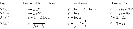
Example 5.2 The Windmill Data
A research engineer is investigating the use of a windmill to generate electricity. He has collected data on the DC output from his windmill and the corresponding wind velocity. The data are plotted in Figure 5.5 and listed in Table 5.5.
Inspection of the scatter diagram indicates that the relationship between DC output (y) and wind velocity (x) may be nonlinear. However, we initially fit a straight-line model to the data. The regression model is
![]()
The summary statistics for this model are R2 = 0.8745, MSRes = 0.0557, and F0 = 160.26 (the P value is <0.0001). Column A of Table 5.6 shows the fitted values and residuals obtained from this model. In Table 5.6 the observations are arranged in order of increasing wind speed. The residuals show a distinct pattern, that is, they move systematically from negative to positive and back to negative again as wind speed increases.
A plot of the residuals versus ŷi is shown in Figure 5.6. This residual plot indicates model inadequacy and implies that the linear relationship has not captured all of the information in the wind speed variable. Note that the curvature that was apparent in the scatter diagram of Figure 5.5 is greatly amplified in the residual plot. Clearly some other model form must be considered.
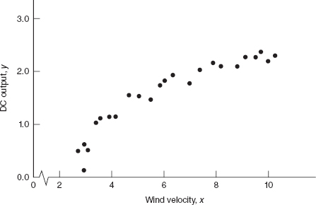
Figure 5.5 Plot of DC output y versus wind velocity x for the windmill data.
TABLE 5.5 Observed Values yi and Regressor Variable xi for Example 5.2

Figure 5.6 Plot of residuals ei versus fitted values ŷi for the windmill data.
We might initially consider using a quadratic model such as
![]()
to account for the apparent curvature. However, the scatter diagram Figure 5.5 suggests that as wind speed increases, DC output approaches an upper limit of approximately 2.5. This is also consistent with the theory of windmill operation. Since the quadratic model will eventually bend downward as wind speed increases, it would not be appropriate for these data. A more reasonable model for the windmill data that incorporates an upper asymptote would be
![]()
Figure 5.7 is a scatter diagram with the transformed variable x′ = 1/x. This plot appears linear, indicating that the reciprocal transformation is appropriate. The fitted regression model is
![]()
The summary statistics for this model are R2 = 0.9800, MSRes = 0.0089, and F0 = 1128.43 (the P value is <0.0001).
The fitted values and corresponding residuals from the transformed model are shown in column B of Table 5.6. A plot of R-student values from the transformed model versus ŷ is shown in Figure 5.8. This plot does not reveal any serious problem with inequality of variance. Other residual plots are satisfactory, and so because there is no strong signal of model inadequacy, we conclude that the transformed model is satisfactory.

Figure 5.7 Plot of DC output versus x′ = 1/x for the windmill data.
TABLE 5.6 Observations yi Ordered by Increasing Wind Velocity, Fitted Values ŷi, and Residuals ei for Both Models for Example 5.2


Figure 5.8 Plot of R-student values ti versus fitted values ŷi for the transformed model for the windmill data.
5.4 ANALYTICAL METHODS FOR SELECTING A TRANSFORMATION
While in many instances transformations are selected empirically, more formal, objective techniques can be applied to help specify an appropriate transformation. This section will discuss and illustrate analytical procedures for selecting transformations on both the response and regressor variables.
5.4.1 Transformations on y: The Box-Cox Method
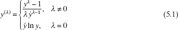
Suppose that we wish to transform y to correct nonnormality and/or nonconstant variance. A useful class of transformations is the power transformation yλ, where λ is a parameter to be determined (e.g., λ = ½ means use √y as the response). Box and Cox [1964] show how the parameters of the regression model and λ can be estimated simultaneously using the method of maximum likelihood.
In thinking about the power transformation yλ a difficulty arises when λ = 0; namely, as λ approaches zero, yλ approaches unity. This is obviously a problem, since it is meaningless to have all of the response values equal to a constant. One approach to solving this difficulty (we call this a discontinuity at λ = 0) is to use (yλ – 1)/λ as the response variable. This· solves the discontinuity problem, because as λ tends to zero, (yλ – 1)/λ goes to a limit of ln y. However, there is still a problem, because as λ changes, the values of (yλ – 1)/λ change dramatically, so it would be difficult to compare model summary statistics for models with different values of λ.
The appropriate procedure is to use
where ![]() is the geometric mean of the observations, and fit the model
is the geometric mean of the observations, and fit the model
by least squares (or maximum likelihood). The divisor ![]() turns out to be related to the Jacobian of the transformation converting the response variable y into y(λ). It is, in effect, a scale factor that ensures that residual sums of squares for models with different values of λ are comparable.
turns out to be related to the Jacobian of the transformation converting the response variable y into y(λ). It is, in effect, a scale factor that ensures that residual sums of squares for models with different values of λ are comparable.
Computational Procedure The maximum-likelihood estimate of λ corresponds to the value of λ for which the residual sum of squares from the fitted model SSRes(λ) is a minimum. This value of λ is usually determined by fitting a model to y(λ) for various values of λ, plotting the residual sum of squares SSRes(λ) versus λ, and then reading the value of λ that minimizes SSRes(λ) from the graph. Usually 10–20 values of λ are sufficient for estimation of the optimum value. A second iteration can be performed using a finer mesh of values if desired. As noted above, we cannot select λ by directly comparing residual sums of squares from the regressions of yλ on x because for each λ the residual sum of squares is measured on a different scale. Equation (5.1) scales the responses so that the residual sums of squares are directly comparable. We recommend that the analyst use simple choices for λ, as the practical difference in the fits for λ = 0.5 and λ = 0.596 is likely to be small, but the former is much easier to interpret.
Once a value of λ is selected, the analyst is now free to fit the model using yλ as the response if λ ≠ 0. If λ = 0, then use ln y as the response. It is entirely acceptable to use y(as the response if) as the response for the final model—this model will have a scale difference and an origin shift in comparison to the model using yas the response if (or ln y). In our experience, most engineers and scientists prefer using yλ (or ln y) as the response.
An Approximate Confidence Interval for λ We can also find an approximate CI for the transformation parameter λ. This CI can be useful in selecting the final value for λ; for example, if ![]() is the minimizing value for the residual sum of squares, but if λ = 0.5 is in the CI, then one might prefer to use the square-root transformation on the basis that it is easier to explain. Furthermore, if λ = 1 is in the CI, then no transformation may be necessary.
is the minimizing value for the residual sum of squares, but if λ = 0.5 is in the CI, then one might prefer to use the square-root transformation on the basis that it is easier to explain. Furthermore, if λ = 1 is in the CI, then no transformation may be necessary.
In applying the method of maximum likelihood to the regression model, we are essentially maximizing
or equivalently, we are minimizing the residual-sum-of-squares function SSRes(λ). An approximate 100(1 – α) percent CI for λ consists of those values of λ that satisfy the inequality
where χ2α,1 is the upper α percentage point of the chi-square distribution with one degree of freedom. To actually construct the CI, we would draw, on a plot of L(λ) versus λ a horizontal line at height
![]()
on the vertical scale. This line would cut the curve of L(λ) at two points, and the location of these two points on the λ axis defines the two end points of the approximate CI. If we are minimizing the residual sum of squares and plotting SSRes(λ) versus λ, then the line must be plotted at height
Remember that ![]() is the value of λ that minimizes the residual sum of squares.
is the value of λ that minimizes the residual sum of squares.
In actually applying the CI procedure, one is likely to find that the factor exp(χ2α,1/n) on the right-hand side of Eq. (5.5) is replaced by either ![]() or
or ![]() or perhaps either
or perhaps either ![]() where ν is the number of residual degrees of freedom. These are based on the expansion of exp(x) = 1 + x + x2/2! + x3/3! + … = 1 + x and the fact that χ21 = z2 ≈ t2ν unless the number of residual degrees of freedom ν is small. It is perhaps debatable whether we should use n or ν, but in most practical cases, there will be very little difference between the CIs that result.
where ν is the number of residual degrees of freedom. These are based on the expansion of exp(x) = 1 + x + x2/2! + x3/3! + … = 1 + x and the fact that χ21 = z2 ≈ t2ν unless the number of residual degrees of freedom ν is small. It is perhaps debatable whether we should use n or ν, but in most practical cases, there will be very little difference between the CIs that result.
Example 5.3 The Electric Utility Data
Recall the electric utility data introduced in Example 5.1. We use the Box-Cox procedure to select a variance-stabilizing transformation. The values of SSRes(λ) for various values of λ are shown in Table 5.7. This display indicates that λ = 0.5 (the square-root transformation) is very close to the optimum value. Notice that we have used a finer “grid” on λ in the vicinity of the optimum. This is helpful in locating the optimum λ more precisely and in plotting the residual-sum-of-squares function.
A graph of the residual sum of squares versus λ is shown in Figure 5.9. If we take λ = 0.5 as the optimum value, then an approximate 95% CI for λ may be found by calculating the critical sum of squares SS* from Eq. (5.5) as follows:
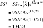
The horizontal line at this height is shown in Figure 5.9. The corresponding values of λ− = 0.26 and λ+ = 0.80 read from the curve give the lower and upper confidence limits for λ, respectively. Since these limits do not include the value 1 (implying no transformation), we conclude that a transformation is helpful. Furthermore, the square-root transformation that was used in Example 5.1 has an analytic justification.
5.4.2 Transformations on the Regressor Variables
Suppose that the relationship between y and one or more of the regressor variables is nonlinear but that the usual assumptions of normally and independently distributed responses with constant variance are at least approximately satisfied. We want to select an appropriate transformation on the regressor variables so that the relationship between y and the transformed regressor is as simple as possible. Box and Tidwell [1962] describe an analylical procedure for determining the form of the transformation on x. While their procedure may be used in the general regression situation, we will present and illustrate its application to the simple linear regression model.
TABLE 5.7 Values of the Residual Sum of Squares for Various Values of λ, Example 5.3
| λ | SSRes (λ) |
| −2 | 34,101.0381 |
| −1 | 986.0423 |
| −0.5 | 291.5834 |
| 0 | 134.0940 |
| 0.125 | 118.1982 |
| 0.25 | 107.2057 |
| 0.375 | 100.2561 |
| 0.5 | 96.9495 |
| 0.625 | 97.2889 |
| 0.75 | 101.6869 |
| 1 | 126.8660 |
| 2 | 1,275.5555 |

Figure 5.9 Plot of residual sum of squares SSRes(λ) versus λ.
Assume that the response variable y is related to a power of the regressor, say ξ = xa, as
where
![]()
and β0, β1, and α are unknown parameters. Suppose that α0 is an initial guess of the constant α. Usually this first guess is α0 = 1, so that ξ = xα0 = x, or that no transformation at all is applied in the first iteration. Expanding about the initial guess in a Taylor series and ignoring terms of higher than first order gives

Now if the term in braces in Eq. (5.6) were known, it could be treated as an additional regressor variable, and it would be possible to estimate the parameters β0, β1, and α in Eq. (5.6) by least squares. The estimate of α could be taken as an improved estimate of the transformation parameter. The term in braces in Eq. (5.6) can be written as
![]()
and since the form of the transformation is known, that is, ξ = xα, we have dξ/dα = x ln x. Furthermore,
![]()
This parameter may be conveniently estimated by fitting the model
by least squares. Then an “adjustment” to the initial guess α0 = 1 may be computed by defining a second regressor variable as w = x ln x, estimating the parameters in
by least squares, giving
and taking
as the revised estimate of α. Note that ![]() is obtained from Eq. (5.7) and
is obtained from Eq. (5.7) and ![]() from Eq. (5.9); generally
from Eq. (5.9); generally ![]() and
and ![]() will differ. This procedure may now be repeated using a new regressor x′ = xα1 in the calculations. Box and Tidwell [1962] note that this procedure usually converges quite rapidly, and often the first-stage result α is a satisfactory estimate of α. They also caution that round-off error is potentially a problem and successive values of α may oscillate wildly unless enough decimal places are carried. Convergence problems may be encountered in cases where the error standard deviation σ is large or when the range of the regressor is very small compared to its mean. This situation implies that the data do not support the need for any transformation.
will differ. This procedure may now be repeated using a new regressor x′ = xα1 in the calculations. Box and Tidwell [1962] note that this procedure usually converges quite rapidly, and often the first-stage result α is a satisfactory estimate of α. They also caution that round-off error is potentially a problem and successive values of α may oscillate wildly unless enough decimal places are carried. Convergence problems may be encountered in cases where the error standard deviation σ is large or when the range of the regressor is very small compared to its mean. This situation implies that the data do not support the need for any transformation.
Example 5.4 The Windmill Data
We will illustrate this procedure using the windmill data in Example 5.2. The scatter diagram in Figure 5.5 suggests that the relationship between DC output (y) and wind speed (x) is not a straight line and that some transformation on x may be appropriate.
We begin with the initial guess α0 = 1 and fit a straight-line model, giving ŷ = 0.1309+0.2411x. Then defining w = x ln x, we fit Eq. (5.8) and obtain
![]()
From Eq. (5.10) we calcnlate
![]()
as the improved estimate of α. Note that this estimate of α is very close to −1, ·so that the reciprocal transformation on x actually used in Example 5.2 is supported by the Box-Tidwell procedure.
To perform a second iteration, we would define a new regressor variable x′ = x−0.92 and fit the model
![]()
Then a second regressor w′ = x′ ln x′ is formed and we fit
![]()
The second-step estimate of α is thus
![]()
which again supports the use of the reciprocal transformation on x.
5.5 GENERALIZED AND WEIGHTED LEAST SQUARES
Linear regression models with nonconstant error variance can also be fitted by the method of weighted least squares. In this method of estimation the deviation between the observed and expected values of yi is multiplied by a weight wi chosen inversely proportional to the variance of yi. For the case of simple linear regression, the weighted least-squares function is
The resulting least-squares normal equations are
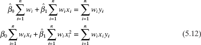
Solving Eq. (5.12) will produce weighted least-squares estimates of β0 and β1.
In this section we give a development of weighted least squares for the multiple regression model. We begin by considering a slightly more general situation concerning the structure of the model errors.
5.5.1 Generalized Least Squares
The assumptions usually made concerning the linear regression model y = Xβ + ε are that E(ε) = 0 and that Varσ2I. As we have observed, sometimes these assumptions are unreasonable, so that we will now consider what modifications to these in the ordinary least-squares procedure are necessary when Var(ε) = σ2V, where V is a known n × n matrix. This situation has an easy interpretation; if V is diagonal but with unequal diagonal elements, then the observations y are uncorrelated but have unequal variances, while if some of the off-diagonal elements of V are nonzero, then the observations are correlated.
When the model is
the ordinary least-squares estimator ![]() is no longer appropriate. We will approach this problem by transforming the model to a new set of observations that satisfy the standard least-squares assumptions. Then we will use ordinary least squares on the transformed data. Since σ2V is the covariance matrix of the errors, V must be nonsingular and positive definite, so there exists an n × n nonsingular symmetric matrix K, where K′K = KK = V. The matrix K is often called the square root of V. Typically, σ2 is unknown, in which case V represents the assumed structure of the variances and covariances among the random errors apart from a constant.
is no longer appropriate. We will approach this problem by transforming the model to a new set of observations that satisfy the standard least-squares assumptions. Then we will use ordinary least squares on the transformed data. Since σ2V is the covariance matrix of the errors, V must be nonsingular and positive definite, so there exists an n × n nonsingular symmetric matrix K, where K′K = KK = V. The matrix K is often called the square root of V. Typically, σ2 is unknown, in which case V represents the assumed structure of the variances and covariances among the random errors apart from a constant.
Define the new variables
so that the regression model y = Xβ + ε becomes K−1y = K−1Xβ + K−1ε, or
The errors in this transformed model have zero expectation, that is, E(g) = K−1E(ε) = 0. Furthermore, the covariance matrix of g is

Thus, the elements of g have mean zero and constant variance and are uncorrelated. Since the errors g in the model (5.15) satisfy the usual assumptions, we may apply ordinary least squares. The least-squares function is
The least-squares normal equations are
and the solution to these equations is
Here ![]() is called the generalized least-squares estimator of β.
is called the generalized least-squares estimator of β.
It is not difficult to show that ![]() is an unbiased estimator of β. The covariance matrix of
is an unbiased estimator of β. The covariance matrix of ![]() is
is
Appendix C.11 shows that ![]() is the best linear unbiased estimator of β. The analysis of variance in terms of generalized least squares is summarized in Table 5.8.
is the best linear unbiased estimator of β. The analysis of variance in terms of generalized least squares is summarized in Table 5.8.
TABLE 5.8 Analysis of Variance for Generalized Least Squares

5.5.2 Weighted Least Squares
When the errors ε are uncorrelated but have unequal variances so that the covariance matrix of ε is

say, the estimation procedure is usually called weighted least squares. Let W = V−1. Since V is a diagonal matrix, W is also diagonal with diagonal elements or weights w1, w2 …, wn. From Eq. (5.18), the weighted least-squares normal equations are
![]()
This is the multiple regression analogue of the weighted least-squares normal equations for simple linear regression given in Eq. (5.12). Therefore,
![]()
is the weighted least-squares estimator. Note that observations with large variances will have smaller weights than observations with small variances.
Weighted least-squares estimates may be obtained easily from an ordinary least-squares computer program. If we multiply each of the observed values for the ith observation (including the 1 for the intercept) by the square root of the weight for that observation, then we obtain a transformed set of data:
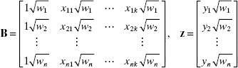
Now if we apply ordinary least squares to these transformed data, we obtain
![]()
the weighted least-squares estimate of β.
Both JMP and Minitab will perform weighted least squares. SAS will do weighted least squares. The user must specify a “weight” variable, for example, w. To perform weighted least squares, the user adds the following statement after the model statement:
weight w;
5.5.3 Some Practical Issues
To use weighted least squares, the weights wi must be known. Sometimes prior knowledge or experience or information from a theoretical model can be used to determine the weights (for an example of this approach, see Weisberg [1985]). Alternatively, residual analysis may indicate that the variance of the errors may be a function of one of the regressors, say Var(εi) = σ2xij, so that wi = 1/xij. In some cases yi is actually an average of ni observations at xi and if all original observations have constant variance σ2, then the variance of yi is Var(yi) = Var(εi) = σ2/ni, and we would choose the weights as wi = ni. Sometimes the primary source of error is measurement error and different observations are measured by different instruments of unequal but known (or well-estimated) accuracy. Then the weights could be chosen inversely proportional to the variances of measurement error. In many practical cases we may have to guess at the weights, perform the analysis, and then reestimate the weights based on the results. Several iterations may be necessary.
Since generalized or weighted least squares requires making additional assumptions regarding the errors, it is of interest to ask what happens when we fail to do this and use ordinary least squares in a situation where Var(ε) = σ2ν with V ≠ I. If ordinary least squares is used in this case, the resulting estimator ![]() is still unbiased. However, the ordinary least-squares estimator is no longer a minimum-variance estimator. That is, the covariance matrix of the ordinary least-squares estimator is
is still unbiased. However, the ordinary least-squares estimator is no longer a minimum-variance estimator. That is, the covariance matrix of the ordinary least-squares estimator is
and the covariance matrix of the generalized least-squares estimator (5.20) gives smaller variances for the regression coefficients. Thus, generalized or weighted least squares is preferable to ordinary least squares whenever V ≠ I.
Example 5.5 Weighted Least Squares
The average monthly income from food sales and the corresponding annual advertising expenses for 30 restaurants are shown in columns a and b of Table 5.9. Management is interested in the relationship between these variables, and so a linear regression model relating food sales y to advertising expense x is fit by ordinary least squares, resulting in ŷ = 49, 443.3838+8.0484x. The residuals from this least-squares fit are plotted against ŷi in Figure 5.10. This plot indicates violation of the constant-variance assumption. Consequently, the ordinary least-squares fit is inappropriate.
TABLE 5.9 Restaurant Food Sales Data

To correct this inequality-of-variance problem, we must know the weights wi. We note from examining the data in Table 5.9 that there are several sets of x values are “near neighbors,” that is, that have approximate repeat points on x. We will assume that these near neighbors are close enough to be considered repeat points and use the variance of the responses at those repeat points to investigate how Var(y) changes with x. Columns c and d of Table 5.9 show the average x value (![]() ) for each cluster of near neighbors and the sample variance of the y's in each cluster. Plotting sy2 against the corresponding
) for each cluster of near neighbors and the sample variance of the y's in each cluster. Plotting sy2 against the corresponding ![]() implies that sy2 increases approximately linearly with
implies that sy2 increases approximately linearly with ![]() . A least-squares fit gives
. A least-squares fit gives

Figure 5.10 Plot of ordinary least-squares residuals versus fitted values, Example 5.5.
![]()
Substituting each xi value into this equation will give an estimate of the variance of the corresponding observation yi. The inverse of these fitted values will be reasonable estimates of the weights wi. These estimated weights are shown in column e of Table 5.9.
Applying weighted least squares to the data using the weights in Table 5.9 gives the fitted model
![]()
We must now examine the residuals to determine if using weighted least squares has improved the fit. To do this, plot the weighted residuals ![]() where ŷi comes from the weighted least-squares fit, against wi½ŷi. This plot is shown in Figure 5.11 and is much improved when compared to the previous plot for the ordinary least-squares fit. We conclude that weighted least squares has corrected the inequality-of-variance problem.
where ŷi comes from the weighted least-squares fit, against wi½ŷi. This plot is shown in Figure 5.11 and is much improved when compared to the previous plot for the ordinary least-squares fit. We conclude that weighted least squares has corrected the inequality-of-variance problem.
Two other points concerning this example should be made. First, we were fortunate to have several near neighbors in the x space. Furthermore, it was easy to identify these clusters of points by inspection of Table 5.9 because there was only one regressor involved. With several regressors visual identification of these clusters would be more difficult. Recall that an analytical procedure for finding pairs of points that are close together in x space was presented in Section 4.5.3. The second point involves the use of a regression equation to estimate the weights. The analyst should carefully check the weights produced by the equation to be sure that they are reasonable. For example, in our problem a sufficiently small x value could result in a negative weight, which is clearly unreasonable.
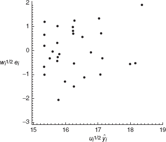
Figure 5.11 Plot of weighted residuals wi½ei versus weighted fitted values wi½ŷi, Example 5.5.
5.6 REGRESSION MODELS WITH RANDOM EFFECTS
5.6.1 Subsampling
Random effects allow the analyst to take into account multiple sources of variability. For example, many people use simple paper helicopters to illustrate some of the basic principles of experimental design. Consider a simple experiment to determine the effect of the length of the helicopter's wings to the typical flight time. There often is quite a bit of error associated with measuring the time for a specific flight of a helicopter, especially when the people who are timing the flights have never done this before. As a result, a popular protocol for this experiment has three people timing each flight to get a more accurate idea of its actual flight time. In addition, there is quite a bit of variability from helicopter to helicopter, particularly in a corporate short course where the students have never made these helicopters before. This particular experiment thus has two sources of variability: within each specific helicopter and between the various helicopters used in the study.
A reasonable model for this experiment is
where m is the number of helicopters, ri is the number of measured flight times for the ith helicopter, yij is the flight time for the jth flight of the ith helicopter, xi is the length of the wings for the ith helicopter, δi is the error term associated with the ith helicopter, and εij is the random error associated with the jth flight of the ith helicopter. The key point is that there are two sources of variability represented by δi and εij. Typically, we would assume that the δis are independent and normally distributed with a mean of 0 and a constant variance σ2δ, that the εijs are independent and normally distributed with mean 0 and constant variance σ2, and that the δis and the εijs are independent. Under these assumptions, the flight times for a specific helicopter are correlated. The flight times across helicopters are independent.
Equation (5.22) is an example of a mixed model that contains fixed effects, in this case the xis, and random effects, in this case the δis and the εijs. The units used for a specific random effect represent a random sample from a much larger population of possible units. For example, patients in a biomedical study often are random effects. The analyst selects the patients for the study from a large population of possible people. The focus of all statistical inference is not on the specific patients selected; rather, the focus is on the population of all possible patients. The key point underlying all random effects is this focus on the population and not on the specific units selected for the study. Random effects almost always are categorical.
The data collection method creates the need for the mixed model. In some sense, our standard regression model y = Xβ + ε is a mixed model with β representing the fixed effects and ε representing the random effects. More typically, we restrict the term mixed model to the situations where we have more than one error term.
Equation (5.22) is the standard model when we have multiple observations on a single unit. Often we call such a situation subsampling. The experimental protocol creates the need for two separate error terms. In most biomedical studies we have several observations for each patient. Once again, our protocol creates the need for two error terms: one for the observation-to-observation differences within a patient and another error term to explain the randomly selected patient-to-patient differences.
In the subsampling situation, the total number of observations in the study, n = Σmi=1 ri. Equation (5.22) in matrix form is
![]()
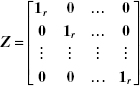
where Z is a n × m “incidence” matrix and δ is a m × 1 vector of random helicopter-to-helicopter errors. The form of Z is

where 1i is a ri × 1 vector of ones. We can establish that
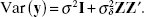
![]()
The matrix ZZ′ is block diagonal with each block consisting of a ri × ri matrix of ones. The net consequence of this model is that one should use generalized least squares to estimate β. In the case that we have balanced data, where there are the same number of observations per helicopter, then the ordinary least squares estimate of β is exactly the same as the generalized least squares estimate and is the best linear unbiased estimate. As a result, ordinary least squares is an excellent way to estimate the model. However, there are serious issues with any inference based on the usual ordinary least squares methodology because it does not reflect the helicopter-to-helicopter variability. This important source of error is missing from the usual ordinary least squares analysis. Thus, while it is appropriate to use ordinary least squares to estimate the model, it is not appropriate to do the standard ordinary least squares inference on the model based on the original flight times. To do so would be to ignore the impact of the helicopter-to-helicopter error term. In the balanced case and only in the balanced case, we can construct exact F and t tests. It can be shown (see Exercise 5.19) that the appropriate error term is based on
![]()
which has m – p degrees of freedom. Basically, this error term uses the average flight times for each helicopter rather than the individual flight times. As a result, the generalized least squares analysis is exactly equivalent to doing an ordinary least squares analysis on the average flight time for each helicopter. This insight is important when using the software, as we illustrate in the next example.
If we do not have balance, then we recommend residual maximum likelihood, also known as restricted maximum likelihood (REML) as the basis for estimation and inference (see Section 5.6.2). In the unbalanced situation there are no best linear unbiased estimates of β. The inference based on REML is asymptotically efficient.
Example 5.6 The Helicopter Subsampling Study
Table 5.10 summarizes data from an industrial short course on experimental design that used the paper helicopter as a class exercise. The class conducted a simple 22 factorial experiment replicated a total of twice. As a result, the experiment required a total of eight helicopters to see the effect of “aspect,” which was the length of the body of a paper helicopter, and “paper,” which was the weight of the paper, on the flight time. Three people timed the each helicopter flight, which yields three flight times for each flight. The variable Rep is necessary to do the proper analysis on the original flight times. The table gives the data in the actual run order.
The Minitab analysis of the original flight times requires three steps. First, we can do the ordinary least squares estimation of the model to get the estimates of the model coefficients. Next, we need to re-analyze the data to get the estimate of the proper error variance. The final step requires us to update the t statistics from the first step to reflect the proper error term.
Table 5.11 gives the analysis for the first step. The estimated model is correct. However, the R2, the t statistics, the F statistics and their associated P values are all incorrect because they do not reflect the proper error term.
The second step creates the proper error term. In so doing, we must use the General Linear Model functionality within Minitab. Basically, we treat the factors and their interaction as categorical. The model statement to generate the correct error term is:
![]()
One then must list rep as a random factor. Table 5.12 gives the results. The proper error term is the mean squared for rep(aspect paper).
TABLE 5.10 The Helicopter Subsampling Data

TABLE 5.11 Minitab Analysis for the First Step of the Helicopter Subsampling Data

TABLE 5.12 Minitab Analysis for the Second Step of the Helicopter Subsampling Data

The third step is to correct the t statistics from the first step. The mean squared residual from the first step is 0.167. The correct error variance is 0.6564. Both of these values are rounded, which is all right, but it will lead to small differences when we do a correct one-step procedure based on the average flight times. Let tj be the t-statistic for the first-step analysis for the jth estimated coefficient, and let tc,j be the corrected statistic given by
![]()
These t statistics have the degrees of freedom associated with rep(aspect paper), which in this case is 4. Table 5.13 gives the correct t statistics and P values. We note that the correct t statistics are smaller in absolute value than for the first-step analysis. This result reflects the fact that the error variance in the first step is too small since it ignores the helicopter-to-helicopter variability. The basic conclusion is that aspect seems to be the only important factor, which is true in both the first-step analysis and the correct analysis. It is important to note, however, that this equivalence does not hold in general. Regressors that appear important in the first-step analysis often are not statistically significant in the correct analysis.
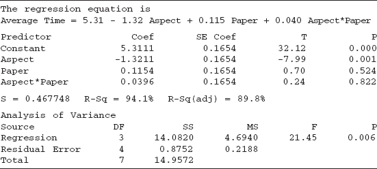
An easier way to do this analysis in Minitab recognizes that we do have a balanced situation here because we have exactly three times for each helicopter's flight. As a result, we can do the proper analysis using the average time for each helicopter flight. Table 5.14 summarizes the data. Table 5.15 gives the analysis from Minitab, which apart from rounding reflects the same values as Table 5.12. We can do a full residual analysis of these data, which we leave as an exercise for the reader.
5.6.2 The General Situation for a Regression Model with a Single Random Effect
The balanced subsampling problem discussed in Section 5.6.1 is common. This section extends these ideas to the more general situation when there is a single random effect in our regression model.
For example, suppose an environmental engineer postulates that the amount of a particular pollutant in lakes across the Commonwealth of Virginia depends upon the water temperature. She takes water samples from various randomly selected locations for several randomly selected lakes in Virginia. She records the water temperature at the time of the sample was taken. She then sends the water sample to her laboratory to determine the amount of the particular pollutant present. There are two sources of variability: location-to-location within a lake and lake-to-lake. This point is important. A heavily polluted lake is likely to have much higher amount of the pollutant across all of its locations than a lightly polluted lake.
TABLE 5.13 Correct t Statistics and P Values for the Helicopter Subsampling Data

TABLE 5.14 Average Flight Times for the Helicopter Subsampling Data
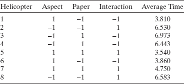
TABLE 5.15 Final Minitab Analysis for the Helicopter Experiment in Table 5.14
The model given by Equation (5.22) provides a basis for analyzing these data. The water temperature is a fixed regressor. There are two components to the variability in the data: the random lake effect and the random location within the lake effect. Let σ2 be the variance of the location random effect, and let σ2δ be the variance of the lake random effect.
Although we can use the same model for this lake pollution example as the subsampling experiment, the experimental contexts are very different. In the helicopter experiment, the helicopter is the fundamental experimental unit, which is the smallest unit to which we can apply the treatment. However, we realize that there is a great deal of variability in the flight times for a specific helicopter. Thus, flying the helicopter several times gives us a better idea about the typical flying time for that specific helicopter. The experimental error looks at the variability among the experimental units. The variability in the flying times for a specific helicopter is part of the experimental error, but it is only a part. Another component is the variability in trying to replicate precisely the levels for the experimental factors. In the subsampling case, it is pretty easy to ensure that the number of subsamples (in the helicopter case, the flights) is the same, which leads to the balanced case.
In the lake pollution case, we have a true observational study. The engineer is taking a single water sample at each location. She probably uses fewer randomly selected locations for smaller lakes, and more randomly selected lakes from largerlakes. In addition, it is not practical for her to sample from every lake in Virginia. On the other hand, it is very straightforward for her to select randomly a series of lakes for testing. As a result, we expect to have different number of locations for each lake; hence, we expect to see an unbalanced situation.
We recommend the use of REML for the unbalanced case. REML is a very general method for analysis of statistical models with random effects represented by the model terms δi and εij in Equation (5.22). Many software packages use REML to estimate the variance components associated with the random effects in mixed models like the model for the paper helicopter experiment. REML then uses an iterative procedure to pursue a weighted least squares approach for estimating the model. Ultimately, REML uses the estimated variance components to perform statistical tests and construct confidence intervals for the final estimated model.
REML operates by dividing the parameter estimation problem into two parts. In the first stage the random effects are ignored and the fixed effects are estimated, usually by ordinary least squares. Then a set of residuals from the model is constructed and the likelihood function for these residuals is obtained. In the second stage the maximum likelihood estimates for the variance components are obtained by maximizing the likelihood function for the residuals. The procedure then takes the estimated variance components to produce an estimate of the variance of y, which it then uses to reestimate the fixed effects. It then updates the residuals and the estimates of the variance components. The procedure continues to some convergence criterion. REML always assumes that the observations are normally distributed because this simplifies setting up the likelihood function.
REML estimates have all the properties of maximum likelihood. As a result, they are asymptotically unbiased and minimum variance. There are several ways to determine the degrees of freedom for the maximum likelihood estimates in REML, and some controversy about the best way to do this, but a full discussion of these issues is beyond the scope of this book. The following example illustrates the use of REML for a mixed effects regression model.

Figure 5.12 JMP results for the delivery time data treating city as a random effects.
Example 5.7 The Delivery Time Data Revisited
We introduced the delivery time data in Example 3.1. In Section 4.2.6 we observed that the first seven observations were collected from San Diego, observations 8–17 from Boston, observations 18–23 from Austin, and observations 24 and 25 from Minneapolis.
It is not unreasonable to assume that the cities used in this study represent a random sample of cities across the country. Ultimately, our interest is the impact of the number of cases deliveryed and the distance required to make the delivery on the delivery times over the entire country. As a result, a proper analysis needs to consider the impact of the random city effect on this analysis.
Figure 5.12 summarizes the analysis from JMP. We see few differences in the parameter estimates between the mixed model analysis that did not include the city's factor, given in Example 3.1. The P values for cases and distance are larger but only slightly so. The intercept P value is quite a bit larger. Part of this change is due to the significant decrease in the effective degrees of freedom for the intercept effect as the result of using the city information. The plot of the actual delivery times versus the predicted shows that the model is reasonable. The variance component for city is approximately 2.59. The variance for the residual error is 8.79. In the original analysis of Example 3.1 is 10.6. Clearly, part of the variability from the Example 3.1 analysis considered purely random is due to systematic variability due to the various cities, which the REML reflects through the cities' variance component.
The SAS code to analyze these data is:
proc mixed cl;
    class city;
    model time = cases distance / ddfm = kenwardroger s;
    random city;
run;
The following R code assumes that the data are in the object deliver. Also, one must load the package nlme in order to perform this analysis.
deliver.model < - lme(time~cases+dist, random =~1|city,
data = deliver) print(deliver.model)
R reports the estimated standard deviations rather than the variances. As a result, one needs to square the estimates to get the same results as SAS and JMP
5.6.3 The Importance of the Mixed Model in Regression
Classical regression analysis always has assumed that there is only one source of variability. However, the analysis of many important experimental designs often has required the use of multiple sources of variability. Consequently, analysts have been using mixed models for many years to analyze experimental data. However, in such cases, the investigator typically planned a balanced experiment, which made for a straightforward analysis. REML evolved as a way to deal with imbalance primarily for the analysis of variance (ANOVA) models that underlie the classical analysis of experimental designs.
Recently, regression analysts have come to understand that there often are multiple sources of error in their observational studies. They have realized that classical regression analysis falls short in taking these multiple error terms in the analysis. They have realized that the result often is the use of an error term that understates the proper variability. The resulting analyses have tended to identify more significant factors than the data truly justifies.
We intend this section to be a short introduction to the mixed model in regression analysis. It is quite straightforward to extend what we have done here to more complex mixed models with more error terms. We hope that this presentation will help readers to appreciate the need for mixed models and to see how to modify the classical regression model and analysis to accommodate more complex error structures. The modification requires the use of generalized least squares; however, it is not difficult to do.
PROBLEMS
5.1 Byers and Williams (“Viscosities of Binary and Ternary Mixtures of Polyaromatic Hydrocarbons,” Journal of Chemical and Engineering Data, 32, 349–354, 1987) studied the impact of temperature (the regressor) on the viscosity (the response) of toluene-tetralin blends. The following table gives the data for blends with a 0.4 molar fraction of toluene.
| Temperature (°C) | Viscosity (mPa · s) |
| 24.9 | 1.133 |
| 35.0 | 0.9772 |
| 44.9 | 0.8532 |
| 55.1 | 0.7550 |
| 65.2 | 0.6723 |
| 75.2 | 0.6021 |
| 85.2 | 0.5420 |
| 95.2 | 0.5074 |
- Plot a scatter diagram. Does it seem likely that a straight-line model will be adequate?
- Fit the straight-line model. Compute the summary statistics and the residual plots. What are your conclusions regarding model adequacy?
- Basic principles of physical chemistry suggest that the viscosity is an exponential function of the temperature. Repeat part b using the appropriate transformation based on this information.
5.2 The following table gives the vapor pressure of water for various temperatures.
| Temperature (°K) | Vapor Pressure (mm Hg) |
| 273 | 4.6 |
| 283 | 9.2 |
| 293 | 17.5 |
| 303 | 31.8 |
| 313 | 55.3 |
| 323 | 92.5. |
| 333 | 149.4 |
| 343 | 233.7 |
| 353 | 355.1 |
| 363 | 525.8 |
| 373 | 760.0 |
- Plot a scatter diagram. Does it seem likely that a straight-line model will be adequate?
- Fit the straight-line model. Compute the summary statistics and the residual plots. What are your conclusions regarding model adequacy?
- From physical chemistry the Clausius-Clapeyron equation states that

Repeat part b using the appropriate transformation based on this information.
5.3 The data shown below present the average number of surviving bacteria in a canned food product and the minutes of exposure to 300°F heat.
| Number of Bacteria | Minutes of Exposure |
| 175 | 1 |
| 108 | 2 |
| 95 | 3 |
| 82 | 4 |
| 71 | 5 |
| 50 | 6 |
| 49 | 7 |
| 31 | 8 |
| 28 | 9 |
| 17 | 10 |
| 16 | 11 |
| 11 | 12 |
- Plot a scatter diagram. Does it seem likely that a straight-line model will be adequate?
- Fit the straight-line model. Compute the summary statistics and the residual plots. What are your conclusions regarding model adequacy?
- Identify an appropriate transformed model for these data. Fit this model to the data and conduct the usual tests of model adequacy.
5.4 Consider the data shown below. Construct a scatter diagram and suggest an appropriate form for the regression model. Fit this model to the data and conduct the standard tests of model adequacy.
![]()
5.5 A glass bottle manufacturing company has recorded data on the average number of defects per 10,000 bottles due to stones (small pieces of rock embedded in the bottle wall) and the number of weeks since the last furnace overhaul. The data are shown below.

- Fit a straight-line regression model to the data and perform the standard tests for model adequacy.
- Suggest an appropriate transformation to eliminate the problems encountered in part a. Fit the transformed model and check for adequacy.
5.6 Consider the fuel consumption data in Table B.18. For the purposes of this exercise, ignore regressor x1. Recall the thorough residual analysis of these data from Exercise 4.27. Would a transformation improve this analysis Why or why not? If yes, perform the transformation and repeat the full analysis.
5.7 Consider the methanol oxidation data in Table B.20. Perform a thorough analysis of these data. Recall the thorough residual analysis of these data from Exercise 4.29. Would a transformation improve this analysis? Why or why not? If yes, perform the transformation and repeat the full analysis.
5.8 Consider the three models
- y = β0 + β1(1/x) + ε
- 1/y = β0 + β1x + ε
- y = x/(β0 – β1x) + ε
All of these models can be linearized by reciprocal transformations. Sketch the behavior of y as a function of x. What observed characteristics in the scatter diagram would lead you to choose one of these models?
5.9 Consider the clathrate formation data in Table B.8.
- Perform a thorough residual analysis of these data.
- b. Identify the most appropriate transformation for these data. Fit this model and repeat the residual analysis.
5.10 Consider the pressure drop data in Table B.9.
- Perform a thorough residual analysis of these data.
- Identify the most appropriate transformation for these data. Fit this model and repeat the residual analysis.
5.11 Consider the kinematic viscosity data in Table B.10.
- Perform a thorough residual analysis of these data.
- Identify the most appropriate transformation for these data. Fit this model and repeat the residual analysis.
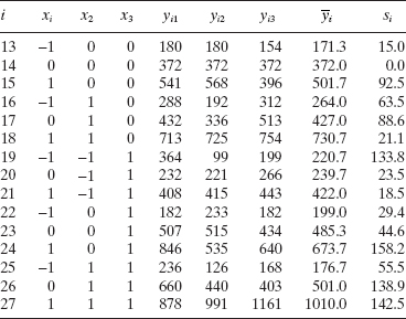
5.12 Vining and Myers (“Combining Taguchi and Response Surface Philosophies: A Dual Response Approach,” Journal of Quality Technology, 22, 15–22, 1990) analyze an experiment, which originally appeared in Box and Draper [1987]. This experiment studied the effect of speed (x1), pressure (x2), and distance (x3) on a printing machine's ability to apply coloring inks on package labels. The following table summarizes the experimental results.

- Fit an appropriate modal to each respone and conduct the residual analysis.
- Use the sample variances as the basis for weighted least-squares estimation of the original data (not the sample means).
- Vining and Myers suggest fitting a linear model to an appropriate transformation of the sample variances. Use such a model to develop the appropriate weights and repeat part b.
5.13 Schubert et al. (“The Catapult Problem: Enhanced Engineering Modeling Using Experimental Design,” Quality Engineering, 4, 463–473, 1992) conducted an experiment with a catapult to determine the effects of hook (x1), arm length (x2), start angle (x3), and stop angle (x4) on the distance that the catapult throws a ball. They threw the ball three times for each setting of the factors. The following table summarizes the experimental results.

- Fit a first-order regression model to the data and conduct the residual analysis.
- Use the sample variances as the basis for weighted least-squares estimation of the original data (not the sample means).
- Fit an appropriate model to the sample variances (note: you will require an appropriate transformation!). Use this model to develop the appropriate weights and repeat part b.
5.14 Consider the simple linear regression model yi = β0 + β1xi + εi, where the variance of εi is proportional to xi2, that is, Var(εi) = σ2x2i.
- Suppose that we use the transformations y′ = y/x and x′ = l/x. Is this a variance-stabilizing transformation?
- What are the relationships between the parameters in the original and transformed models?
- Suppose we use the method of weighted least squares with wi = 1/xi2. Is this equivalent to the transformation introduced in part a?
5.15 Suppose that we want to fit the no-intercept model y = βx + ε using weighted least squares. Assume that the observations are uncorrelated but have unequal variances.
- Find a general formula for the weighted least-squares estimator of β.
- What is the variance of the weighted least-squares estimator?
- Suppose that Var(yi) = cxi, that is, the variance of yi is proportional to the corresponding xi. Using the results of parts a and b, find the weighted least-squares estimator of β and the variance of this estimator.
- Suppose that (yi) = cxi2, that is, the variance of yi is proportional to the square of the corresponding xi. Using the results of parts a and b, find the weighted least-squares estimator of β and the variance of this estimator.
5.16 Consider the model
![]()
where E(ε) = 0 and Var(ε) = σ2V. Assume that σ2 and V are known. Derive an appropriate test statistic for the hypotheses
![]()
Give the distribution under both the null and alternative hypotheses.
5.17 Consider the model
![]()
where E(ε) = 0 and Var(ε) = σ2V. Assume that V is known but not σ2. Show that
![]()
is an unbiased estimate of σ2.
5.18 Table B.14 contains data on the transient points of an electronic inverter. Delete the second observation and use x1 – x4 as regressors. Fit a multiple regression model to these data.
- Plot the ordinary residuals, the studentized residuals, and R-student versus the predicted response. Comment on the results.
- Investigate the utility of a transformation on the response variable. Does this improve the model?
- In addition to a transformation on the response, consider transformations on the regressors. Use partial regression or partial residual plots as an aid in this study.
5.19 Consider the following subsampling model:
![]()
where m is the number of helicopters, r is the number of measured flight times for each helicopter, yij is the flight time for the jth flight of the ith helicopter, xi is the length of the wings for the ith helicopter, δi is the error term associated with the ith helicopter, and εij is the random error associated with the jth flight of the ith helicopter. Assume that the δis are independent and normally distributed with a mean of 0 and a constant variance σδ2, that the εijs are independent and normally distributed with mean 0 and constant variance σ2, and that the δis and the εijs are independent. The total number of observations in this study is ![]() . This model in matrix form is
. This model in matrix form is
![]()
where Z is a n × m “incidence” matrix and δ is a m × 1 vector of random helicopter-to-helicopter errors. The form of Z is
where 1r is a r × 1 vector of ones.
- Show that
- Show that the ordinary least squares estimates of β are the same as the generalized least squares estimates.
- Derive the appropriate error term for testing the regression coefficients.
5.20 The fuel consumption data in Appendix B.18 is actually a subsampling problem. The batches of oil are divided into two. One batch went to the bus, and the other batch went to the truck. Perform the proper analysis of these data.
5.21 A construction engineer studied the effect of mixing rate on the tensile strength of portland cement. From each batch she mixed, the engineer made four test samples. Of course, the mix rate was applied to the entire batch. The data follow. Perform the appropriate analysis.

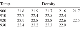
5.22 A ceramic chemist studied the effect of four peak kiln temperatures on the density of bricks. Her test kiln could hold five bricks at a time. Two samples, each from different peak temperatures, broke before she could test their density. The data follow. Perform the appropriate analysis.
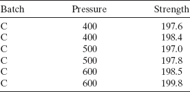
5.23 A paper manufacturer studied the effect of three vat pressures on the strength of one of its products. Three batches of cellulose were selected at random from the inventory. The company made two production runs for each pressure setting from each batch. As a result, each batch produced a total of six production runs. The data follow. Perform the appropriate analysis.

5.24 French and Schultz (“Water Use Efficiency of Wheat in a Mediterranean-type Environment, I The Relation between Yield, Water Use, and Climate,” Australian Journal of Agricultural Research, 35, 743–64) studied the impact of water use on the yield of wheat in Australia. The data below are from 1970 for several locations assumed to be randomly selected for this study. The response, y, is the yield of what in kg/ha. The regressors are:
- x1 the amount of rain in mm for the period October to April.
- x2 is the number of days in the growing season.
- x3 is the amount of rain in mm during the growing season.
- x4 is the water use in mm for the growing season.
- x5 is the pan evaporation in mm during the growing season.
Perform a thorough analysis of these data.
