Closed Economy Model

We begin by assuming that the economy produces output described by a linear homogenous production function:

(7.1)

where

1. L = quantity of labor services employed
2. K = index of real capital²

Per capita output q = Q/L is then a function of capital-labor ratio k = K/L:

(7.2)

where

1. f ′(k) > 0
2. f ″(k) < 0, for all k > 0

Under full employment conditions, the rate of return to capital (the rate of profit of business firms), r, and the wage rate, w, are given by:

(7.3)

(7.4)

The macroeconomy is made up of firms and households. Equity shares to all capital stock represent the ownership claim of households. In Islamic profit-sharing arrangements, business firms exercise direct control over capital by employing it with labor. Households receive income in the form of wages for labor and returns on their equity shares. They divide their income between consumption and savings (to increase their equity holdings). Aggregate demand is composed of household consumption and the level of investment planned by business firms. National income is equal to the returns of the factors of production, which in turn determines the level of actual aggregate demand, consumption, and investment. When planned and actual aggregate demands are equal, the economy is said to be in short-run equilibrium, and a level of aggregate demand corresponding to such an equilibrium level determines the rate of capital accumulation.

Assuming homogenous quantities of labor and capital and that the aggregate behavior of households and business in the economy can be explained in terms of a representative household and business firm, aggregate income, Y, is given by:

(7.5)

where

1. W = wages bill (total wage payments)
2. D = dividends
3. G = expected capital gains

The value of the equity shares held by households is:

(7.6)

where

1. P^e = price of shares
2. E = number of shares

The rate of return to equity is expressed as:

(7.7)

Demand for new equity shares (i.e., the number of new shares desired by households) is given by:

(7.8)

where

1. E^D = dE^D
2. S = savings of households, which is given by:

(7.9)

where

1. s(r^m) = average propensity to save and is a positive function of the rate of return

Aggregate output is distributed as:

(7.10)

where

1. R = portion of profits retained by firms for additional investment

The supply of new shares to be issued by firms is given by:

(7.11)

where

1. E^S = dE^S
2. I = desired investment by firms

Investment is determined by a marginal efficiency schedule (Lucas-Treadway-Uzawa type) and the Penrose function

(7.12)

where

1. z = growth rate of total capital
2. I = I/K

The Penrose function can be interpreted in terms of the marginal cost of investment. The relationship between the investment-capital ratio and the rate of capital accumulation—that is, i = i(z)—requires that

(7.13)

The conditions in equation 7.13 reflect the scarcity of entrepreneurship, investment increases as the real rate of return to real capital increases, and the fact that the marginal cost of investment is increasing.

The optimum level of z, the rate of increase in capital, is a function of the marginal product of capital (the rate of profit), r, and the market rate of return to equity, r^m, prevailing in the equity market. Since i = i(z) and z = z(r, r^m) then:

(7.14)

(7.15)

(7.16)

Equations 7.14 and 7.15 are graphically represented in Figure 7.1 for a given rate of profit r. The rate of capital accumulation z(r, r^m) can be positive or negative, depending on whether the market rate of return is smaller or larger than the rate of profit, r. Also, at a given rate of profit, firms undertake additional investment depending on the magnitude of the market rate of return to equity relative to the rate of profit. In an efficient equity market, no firm will be able to attract financing for its investment projects that do not promise to yield a rate of return at least as large as the prevailing market rate of return on shares.

In an economy just described, the equilibrium condition for the goods market is:

(7.17)

The labor market is in equilibrium when there is full employment, that is:

(7.18)

where

1. N = quantity of labor employed

The labor force is assumed to grow at a rate n and capital accumulation at a rate z, defined relative to the investment-capital ratio i through the Penrose curve. The equity market is in equilibrium when:

(7.19)

and per capita output is given by equation 7.2 as q = f(k). National income is defined as:

(7.20)

Dividing equation 7.20 by N to convert into per capita terms yields:

(7.21)

If we assume that capital gains, G, always reflect retained profits, output will equal national income, as in:

(7.22)

The short-run equilibrium for this economy requires that:

(7.23)

In terms of investment-capital ratio and savings per unit of capital (as well as in per capita terms):

(7.24)

In other words, planned savings must equal planned investment. Equilibrium is attained at a market rate of return, r^m, that equates the level of investment per unit of real capital desired by the firms and the amount of savings per unit of real capital that households are willing to save at the market rate. Figure 7.2 is a graphic representation of investment and saving schedules of equation 7.24. The vertical axis shows the market rate of return, and the horizontal axis shows the desired investment or desired saving per unit of capital. The intersection of the two curves II and SS determines the equilibrium market rate of return. While a change in the market rate of return causes a movement along the curves, a change in the rate of profit, r, causes a shift of the curves. An increase in the capital-labor ratio, k, reduces the marginal product of capital, r (the rate of profit), resulting in a shift of II downward and to the left. The same increase in k reduces average product y/k of capital, causing an upward shift in the SS curve. As a result, investment declines but the market rate of return may or may not decline, depending on the way the two curves shift.

The long-run equilibrium of the system depends only on the rate of growth of the labor force, n. The system will remain at a steady state if, and only if, the rate of investment per unit of capital is at a level i(n), which corresponds to the exogenously given rate of growth of labor, n. The dynamics of the economy is described by the differential equation:

(7.25)

Designating the steady-state level of capital-labor ratio as k*, whenever k is lower than its long-run equilibrium level k*, then the capital-labor ratio increases; that is, k > 0. If k is at a higher level than k*, then k < 0 and the capital-labor ratio declines. The long-run equilibrium level of the capital-labor ratio k* is determined by the long-run equilibrium levels of investment and savings from the equations 7.26 and 7.27:

(7.26)

(7.27)

where

1. r* = long-run equilibrium market rate of return
2. y* = f(k*) and r* = f′(k*) = long-run equilibrium levels of income and profit rates respectively
3. i(n) = equilibrium rate of investment corresponding to the rate of growth of labor, n

Equations 7.26 and 7.27 state that there is a pair of rates of return, and r*, that equate the long-run desired levels of investment and savings per unit of capital. As shown in Figure 7.3, the intersection of desired savings per unit of capital and desired investment per capita determines the long-run equilibrium market rate of return and the capital-labor ratio. The equilibrium conditions (7.26) and (7.27) convey the fact that for any market rate of return (r*) above its long-run equilibrium level, , the rate of profit (r*) must also increase (thus k* must decrease) in order for investment to be maintained at its long-run equilibrium level i(n). Also, an increase in the market rate of return above its long-run equilibrium level must be accompanied by a higher capital-labor ratio (k*) and thus a lower average productivity of capital (y*/k*) in order for savings to equal the long-run equilibrium level of investment i(n). The long-run equilibrium of the economy can be determined once the production function, consumption-saving behavior, investment function (the Penrose curve), and rate of growth of labor (n) are specified.

The important implication of this analysis is that the assumption of a fixed and predetermined rate of interest is not necessary either for the determination of savings-investment behavior or for the existence of a long-run equilibrium for the economy. While it is true that the existence of a rate of time preference may be needed to determine the equilibrium consumption-savings behavior in the economy, and while its necessity or existence in an Islamic economy cannot be denied (nor is there any basis for rejecting its existence on the basis of the Quran and the ahadeeth), there is no strong theoretic justification for assuming that the rate of time preference is fixed, predetermined, and equal to the market rate of interest.³ One could easily and without loss of generality assume that the rate of time preference (discount rate)is equal to the market rate of return on equity shares (in which the rate of time preference is equal to the marginal product of capital).⁴

Open Economy Model

To analyze the consequences of opening a noninterest economy to trade in goods and assets, the closed economy model in the previous section can be used in modified and simplified form. Money is introduced as an additional asset with zero nominal rate of return. Retained earnings can be dropped by assuming that holding shares in a firm that is retaining earnings is equivalent to using these earnings to buy new shares in the firm. The number of shares is assumed equal to the number of units of capital goods so that E = K. Because of our interest in the effects of trade in equity shares, the aggregate supply is assumed to be a function of capital, that is,

(7.28)

The rate of return to equity shares is now defined as

where

1. P = price level
2. P_E = nominal price of shares
3. F′P = value of marginal product of capital

Defining the real price of shares as becomes the rate of return in real terms:

(7.29)

which along with assumptions on capital gains and profits modifies equation 7.15 to become i = i(r). Since by definition and capital stock is given in the short run, investment becomes a function of r and K as:

(7.30)

Real wealth is defined as , where m = MP is the stock of real balances. In searching for an optimal portfolio, individuals adjust their holding of real cash balances and equity until the actual and desired mix of the two assets is equal. Such an equilibrium is represented in Figure 7.4. If the wealth constraint is m₁n₁ instead of mn, the desired mix will be at point B where individuals will attempt to increase their holding of money balances by reducing their equity holdings. Given equation 7.29, as the price of shares decreases, r increases and the slope of m₁n₁ declines, causing it to rotate around point A downward to the right, until it coincides with mn and the original equilibrium is established at point A.

Demand equations for goods, equity, and money are assumed, in real terms, to have the following form⁵:

(7.31)

where

1. i = 1, 2, 3 refer to each market for goods, equity shares, and money
2. m = real income and stock of real balances

The aggregate demand for goods is the sum of consumption and investment. Equilibrium in the three markets is given by:

(7.32)

(7.33)

(7.34)

where

1. Q = aggregate supply
2. PL = demand for money in nominal terms

From these equations, P and r can be determined. Of equations 7.32 to 7.34, only two are independent, given the constraint indicated by the Walras law:

(7.35)

Given the money supply and the level of real capital, and assuming the existence and stability of the system, the price level of goods and the rate of return on equity shares can be determined.⁶ The long-run equilibrium is attained when real capital and money supply do not change. The conditions for long-run equilibrium can be given as when y = AD, E = K, and I = 0. These conditions are satisfied when m = m*, r = r* and K = K*. An asterisk next to the variable designates its long-run equilibrium value.

Assume that the economy is small relative to the rest of the world, that it faces a world price of goods P_f, and that the exchange rate is given by

(7.36)

where

1. P = domestic price level

Concentrating first on trade in goods only, the domestic money supply will increase or decrease corresponding to the balance of trade. The short-run equilibrium is given by

(7.37)

(7.38)

where

1. T = trade balance

From these equations, T and r can be determined. The dynamic structure of the adjustment process is determined by the following pair of differential equations:

(7.39)

(7.40)

If the initial (before trade) domestic price level P is lower than P_f when trade takes place, there is an immediate increase in real balances, which leads to portfolio adjustment in favor of domestic equity shares. There is also a positive trade balance. Recalling portfolio adjustment described in Figure 7.4 and considering equation 7.38, in the first phase of adjustment M becomes positive and K becomes negative, thus lowering the rate of return and increasing investment. Increases in M and K reduce T and K, and the system moves toward its long-run equilibrium position. Once there, all variables attain their steady-state values with new money supply M* and P* = P_f. Under a flexible exchange rate system, the exchange rate adjusts to attain an equilibrium balance of trade and the same pretrade long-run equilibrium will be achieved.

When trade in assets as well as goods is allowed, the short-run equilibrium conditions (7.37) and (7.38) become:

(7.41)

(7.42)

where

1. r_f = world rate of return to equity
2. E_d = domestic holding of domestic equity
3. E_f = foreign holding of domestic equity and equals the difference between domestic capital and the equity claims held by domestic residents

Given K, M, and P_f, then T and E_f can be determined from equations 7.41 and 7.42. If E_f is positive, it means that the country is a debtor; if it is negative, it represents domestic residents' holding of foreign equity claims and the domestic economy is a creditor. It is assumed that the equities being traded internationally are homogenous. If the marginal product of capital is higher in the domestic economy, its equity shares will have a higher price and adjustment in the rate of return to equity shares takes place through adjustment in their prices.

If the domestic rate of return on equities is higher than the world rate, then upon opening of trade, there will be an excess demand for domestic equity, which raises the price of equity and the wealth of domestic households and, along with a reduction in the rate of return, induces an instantaneous portfolio adjustment of the type described in Figure 7.4, where the increase in real value of assets changes the wealth constraint from mn to m₁n₁. The new short-run equilibrium, with a new rate of return equal to r_f, domestic holdings of real cash balances and equities become m and E₁, respectively. Thus the economy exchanges E₁E₀ units of equity for m₀m of real balances with the rest of the world, and the new portfolio equilibrium moves from point A to point B.⁷ With a domestic rate of return greater than r_f, the foreign holding of domestic equities increases initially, that is, E > 0. A lower domestic rate of return and positive M will mean a positive K and a worsening trade balance, but the balance of payments will be positive because of increased demand for money, M > 0. Given a nonoscillating adjustment mechanism, if the initial shock from capital movements is not very strong, the adjustment process will proceed.⁸ An increase in real capital and in payments of return to foreign holdings of domestic equity, which in real terms equals F′E_f, will lead to positive trade accounts.

Considerations of payments for return on foreign holdings of domestic equities, that is, y = F(K) − F′E_f, modifies equations 7.41 and 7.42 to become⁹

(7.43)

(7.44)

Equations 7.43 and 7.44 yield the following simultaneous equation system:

(7.45)

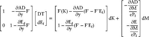
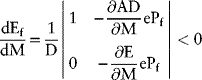
The effects of changes in M and K on the short-run equilibrium values of T and E_f can be determined using equation 7.45, which yields:

(7.46)

(7.47)

(7.48)

(7.49)

and the determinant D is

(7.50)

The results attained in equations 7.46 to 7.49 can be explained as follows: an increase in real capital increases the supply of goods and equity shares, but, because the income effect is normally positive and less than 1, the increase in demand is less than the increase in supply; therefore, foreign demand for goods and equities must increase to restore equilibrium in the market. Thus, the trade balance and foreign holdings of domestic equity respond positively to changes in capital. However, equations 7.48 and 7.49 are negative. The reason is that an increase in money supply increases real balances, and this in turn raises the domestic demand for goods and equity shares. Since the supply of goods and equity do not change, the foreign demand for goods and foreign equity holdings of domestic assets must decline for the markets to clear.¹⁰ Reductions in foreign holdings of domestic equity, of course, lower return payments to foreign holders of equity shares.

The dynamic adjustment equations are:

(7.51)

(7.52)

Equation 7.52 expresses surplus or deficit balance of payment and is the familiar monetary approach to balance of payments. Linearization of differential equations 7.51 and 7.52 yields the following coefficient matrix:

(7.53)

The determinant of this matrix is:

As the trace of equation 7.53 is negative, the equilibrium is locally stable, as shown in Figure 7.5.

The system is also globally stable if the a₂₁ element of equation 7.53 is positive everywhere and its a₂₂ element is negative everywhere. The discriminant of equation 7.53 is (trace) ^2—4 |A|, that is,

Both roots are real and there are no oscillations in the adjustment process.

Given an initial position and the fact that the adjustment path is nonoscillating, the properties of the adjustment process can be explained. The long-run equilibrium is obtained when and . By the Walras law we have

(7.54)

Substituting and in equation 7.54 with given P_f and r_f and the short-run equilibrium conditions, the long-run equilibrium of the economy with trade in goods and assets is

(7.55)

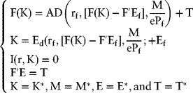
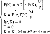
To compare equation 7.55 with the initial position of the economy before trade, we recall the long-run equilibrium without trade, which is as follows:

(7.56)

Clearly, the long-run equilibrium positions of the economy before and after trade are different. When the country begins to trade in goods and equity claims, foreign investors will hold domestic equity shares if the rate of return on domestic equity is higher than the world rate of return on similar assets, and E_f will be positive. But as investors do so, the rate of return declines (and price of equity shares increases), the demand for goods will increase, and the trade account will worsen, T < 0. The balance of payments, however, will be positive because the demand for money has increased and . Lower rates of return increase investment, ; as a result, . In the long run, as and , then . In terms of Figure 7.5, the adjustment process implies that if r > r_f (r < r_f), then the initial position of and are the area below (above) the line and to the left (right) of the line . The adjustment process is reversed if the domestic rate of return on equities is lower than the foreign rate of return on similar assets.

The adjustment process just described can be used to analyze the effects of changes in the exchange rate. Since in the open economy case the quantity of real balances is defined as m = M/eP_f, then any change in the exchange rate will have results analogous to those following changes in the nominal quantity of money.¹¹ Thus, a devaluation is analogous to a one-time reduction in the nominal money supply. Interpreted in this way, no additional derivation is required for examination of the effects of changes in the exchange rate. Equations 7.48 and 7.49, for example, can be used to show the effects of a devaluation on short-run equilibrium values of the trade balance and capital flows. As can be seen from these equations, a devaluation should increase capital inflows, through an increase in foreign ownership of domestic equity, and improve the balance of trade.

Equations 7.48 and 7.49 also imply that the channels through which these effects are transmitted are the asset markets (equity shares and money). A devaluation raises the price level P = eP_f and thereby reduces the value of real balances (therefore, real wealth), inducing an instantaneous portfolio adjustment. Figure 7.6 illustrates the portfolio adjustment triggered by a devaluation. With the initial equilibrium at point D, a devaluation leads to a reduction in real wealth to a point such as C, which then induces an instantaneous portfolio adjustment from C to A when the asset drawdown is divided between equity shares and money so as to achieve portfolio balance. Recall that the system is homogenous of degree zero in the nominal money stock, M, and in the exchange rate, e, and also that the aggregate asset holders' demand for real cash balances, L, is assumed proportional to the value of their equity holdings. As the domestic equity holders reduce their stocks of equities, the price of equities is reduced, thus making them more attractive for exports. However, devaluation reduces aggregate consumption expenditures relative to income, thus leading to an improved balance of trade.

A currency revaluation has the opposite effects since it is as if real balances were raised. There is an excess demand for equity shares, and as a result of an instantaneous portfolio adjustment, part of the increase in real cash balances is exchanged for additional equity holdings. The monetary change, however, does not affect the capital stock, hence the level of output is fixed, but aggregate consumption expenditure increases.¹² Additional equity holding by foreigners of domestic equities leads to an improvement in the capital account (by the amount of the rate of return multiplied by a change in foreign holdings of domestic equities). But at the same time, due to increased consumption, the surplus (deficit) in the balance of trade is reduced (increased). These changes in the capital account reflect the once-and-for-all stock adjustment needed to restore portfolio balance. Much of the adjustment in the short run is channeled through the asset accounts. As the adjustment proceeds, there will be a gradual deaccumulation of assets, which will be reflected in a surplus in the capital account and a deficit in the monetary account. There will also be a gradual improvement in the trade account until the adjustment process comes to an end and the long-run equilibrium is reestablished.