25.3 Shor’s Algorithm
Quantum computers are not yet a reality. The current versions can only handle a few qubits. But, if the great technical problems can be overcome and large quantum computers are built, the effect on cryptography will be enormous. In this section we give a brief glimpse at how a quantum computer could factor large integers, using an algorithm developed by Peter Shor. We avoid discussing quantum mechanics and ask the reader to believe that a quantum computer should be able to do all the operations we describe, and do them quickly. For more details, see, for example, [Ekert-Josza] or [Rieffel-Polak].
What is a quantum computer and what does it do? First, let’s look at what a classical computer does. It takes a binary input, for example, 100010, and gives a binary output, perhaps 0101. If it has several inputs, it has to work on them individually. A quantum computer takes as input a certain number of qubits and outputs some qubits. The main difference is that the input and output qubits can be linear combinations of certain basic states. The quantum computer operates on all basic states in this linear combination simultaneously. In effect, a quantum computer is a massively parallel machine.
For example, think of the basic state as representing three particles, the first in orientation 1 and the last two in orientation 0 (with respect to some basis that will implicitly be fixed throughout the discussion). The quantum computer can take and produce some output. However, it can also take as input a normalized (that is, of length 1) linear combination of basic quantum states such as
and produce an output just as quickly as it did when working with a basic state. After all, the computer could not know whether a quantum state is one of the basic states, or a linear combination of them, without making a measurement. But such a measurement would alter the input. It is this ability to work with a linear combination of states simultaneously that makes a quantum computer potentially very powerful.
Suppose we have a function that can be evaluated for an input by a classical computer. The classical computer asks for an input and produces an output. A quantum computer, on the other hand, can accept as input a sum
( is a normalization factor) of all possible input states and produce the output
where is a longer sequence of qubits, representing both and the value of . (Technical point: It might be notationally better to input in order to have some particles to change to . For simplicity, we will not do this.) So we can obtain a list of all the values of . This looks great, but there is a problem. If you make a measurement, you force the quantum state into the result of the measurement. You get for some randomly chosen , and the other states in the output are destroyed. So, if you are going to look at the list of values of , you’d better do it carefully, since you get only one chance. In particular, you probably want to apply some transformation to the output in order to put it into a more desirable form. The skill in programming a quantum computer is in designing the computation so that the outputs you want to examine appear with much higher probability than the others. This is what is done in Shor’s factorization algorithm.
25.3.1 Factoring
We want to factor . The strategy is as follows. Recall that if we can find (nontrivial) and with , then we have a good chance of factoring (see the factorization method in Subsection 9.4.1). Choose a random and consider the sequence . If , then this sequence will repeat every terms since . If we can measure the period of this sequence (or a multiple of the period), we will have an such that . We therefore want to design our quantum computer so that when we make a measurement on the output, we’ll have a high chance of obtaining the period.
25.3.2 The Discrete Fourier Transform
We need a technique for finding the period of a periodic sequence. Classically, Fourier transforms can be used for this purpose, and they can be used in the present situation, too. Suppose we have a sequence
of length , for some integer . Define the Fourier transform to be
where .
For example, consider the sequence
of length 8 and period 4. The length divided by the period is the frequency, namely 2, which is how many times the sequence repeats. The Fourier transform takes the values
For example, letting , we find that
Since , the terms cancel and we obtain . The nonzero values of occur at multiples of 2, which is the frequency.
Let’s consider another example: . The Fourier transform is
Here the nonzero values of are again at the multiples of the frequency.
In general, if the period is a divisor of , then all the nonzero values of will occur at multiples of the frequency (however, a multiple of the frequency could still yield 0). See Exercise 2.
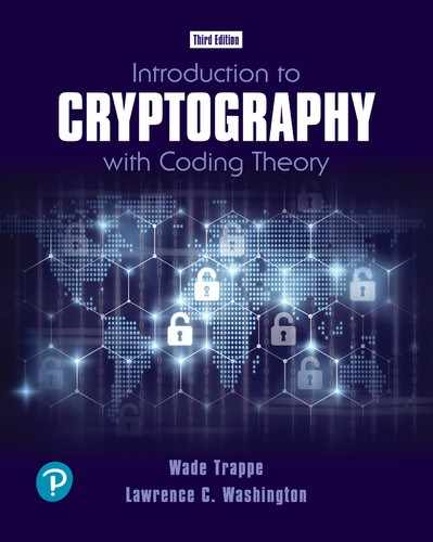
Suppose now that the period isn’t a divisor of . Let’s look at an example. Consider the sequence . It has length 8 and almost has period 3 and frequency 3, but we stopped the sequence before it had a chance to complete the last period. In Figure 25.4, we graph the absolute value of its Fourier transform (these are real numbers, hence easier to graph than the complex values of the Fourier transform). Note that there are peaks at 0, 3, and 5. If we continued to larger values of we would get peaks at . The peaks are spaced at an average distance of 8/3. Dividing the length of the sequence by the average distance yields a period of , which agrees with our intuition.
Figure 25.4 The Absolute Value of a Discrete Fourier Transform
The fact that there is a peak at 0 is not very surprising. The formula for the Fourier transform shows that the value at 0 is simply the sum of the elements in the sequence divided by the square root of the length of the sequence.
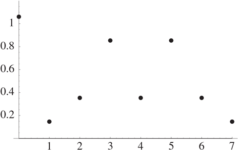
Let’s look at one more example: 1, 0, 0, 0, 0, 1, 0, 0, 0, 0 1, 0, 0, 0, 0, 1. This sequence has 16 terms. Our intuition might say that the period is around 5 and the frequency is slightly more than 3. Figure 25.5 shows the graph of the absolute value of its Fourier transform. Again, the peaks are spaced around 3 apart, so we can say that the frequency is around 3. The period of the original sequence is therefore around 5, which agrees with our intuition.
Figure 25.5 The Absolute Value of a Discrete Fourier Transform
In the first two examples, the period was a divisor of the length (namely, 8) of the sequence. We obtained nonzero values of the Fourier transform only at multiples of the frequency. In these last two examples, the period was not a divisor of the length (8 or 16) of the sequence. This introduced some “noise” into the situation. We had peaks at approximate multiples of the frequency and values close to 0 away from these peaks.
The conclusion is that the peaks of the Fourier transform occur approximately at multiples of the frequency, and the period is approximately the number of peaks. This will be useful in Shor’s algorithm.
25.3.3 Shor’s Algorithm
Choose so that . We start with qubits, all in state 0:
As in the previous section, by changing axes, we can transform the first bit to a linear combination of and , which gives us
We then successively do a similar transformation to the second bit, the third bit, up through the th bit, to obtain the quantum state
Thus all possible states of the qubits are superimposed in this sum. For simplicity of notation, we replace each string of 0s and 1s with its decimal equivalent, so we write
Choose a random number with . We may assume ; otherwise, we have a factor of . The quantum computer computes the function for this quantum state to obtain
(for ease of notation, is used to denote ). This gives a list of all the values of . However, so far we are not any better off than with a classical computer. If we measure the state of the system, we obtain a basic state for some randomly chosen . We cannot even specify which we want to use. Moreover, the system is forced into this state, obliterating all the other values of that have been computed. Therefore, we do not want to measure the whole system. Instead, we measure the value of the second half. Each basic piece of the system is of the form , where represents bits and is represented by bits (since ). If we measure these last bits, we obtain some number , and the whole system is forced into a combination of those states of the form with :
where is whatever factor is needed to make the vector have length 1 (in fact, is the square root of the number of terms in the sum).
Example
At this point, it is probably worthwhile to have an example. Let . (This example might seem simple, but it is the largest that quantum computers using Shor’s algorithm can currently handle. Other algorithms are being developed that can go somewhat farther.) Since , we have . Let’s choose , so we compute the values of to obtain
Suppose we measure the second part and obtain 2. This means we have extracted all the terms of the form to obtain
For notational convenience, and since it will no longer be needed, we drop the second part to obtain
If we now measured this system, we would simply obtain a number such that . This would not be useful.
Suppose we could take two measurements. Then we would have two numbers and with . This would yield . By the factorization method of Subsection 9.4.1, this would give us a good chance of being able to factor . However, we cannot take two independent measurements. The first measurement puts the system into the output state, so the second measurement would simply give the same answer as the first.
Not all is lost. Note that in our example, the numbers in our state are periodic with period 6. In general, the values of are periodic with period , with . So suppose we are able to make a measurement that yields the period. We then have a situation where , so we can hope to factor by the method from Subsection 9.4.1 mentioned above.
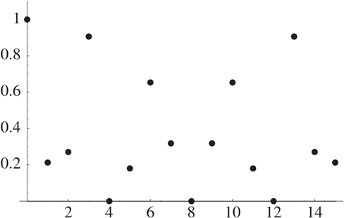
The quantum Fourier transform is exactly the tool we need. It measures frequencies, which can be used to find the period. If happens to be a divisor of , then the frequencies we obtain are multiples of a fundamental frequency , and . In general, is not a divisor of , so there will be some dominant frequencies, and they will be approximate multiples of a fundamental frequency with . This will be seen in the analysis of our example and in Figure 25.6.
Figure 25.6 The Absolute Value of
The quantum Fourier transform is defined on a basic state (with ) by
It extends to a linear combination of states by linearity:
We can therefore apply to our quantum state.
In our example, we compute
and obtain a sum
for some numbers .
The number is given by
which is the discrete Fourier transform of the sequence
Therefore, the peaks of the graph of the absolute value of should correspond to the frequency of the sequence, which should be around . The graph in Figure 25.6 is a plot of .
There are sharp peaks at , , , , , (the ones at 0 and 256 do not show up on the graph since they are centered at one value; see below). These are the dominant frequencies mentioned previously. The values of near the peak at are
The behavior near , , and is similar. At and , we have , while all the nearby values of have .
The peaks are approximately at multiples of the fundamental frequency . Of course, we don’t really know this yet, since we haven’t made any measurements.
Now we measure the quantum state of this Fourier transform. Recall that if we start with a linear combination of states normalized such that , then the probability of of obtaining is . More generally, if we don’t assume , the probability is
In our example,
so if we sample the Fourier transform, the probability is around that we obtain one of , , , . Let’s suppose this is the case; say we get . We know, or at least expect, that 427 is approximately a multiple of the frequency that we’re looking for:
for some . Since , we divide to obtain
Note that . Since we must have , a reasonable guess is that (see the following discussion of continued fractions).
In general, Shor showed that there is a high chance of obtaining a value of with
for some . The method of continued fractions will find the unique (see Exercise 3) value of with satisfying this inequality.
In our example, we take and check that .
We want to use the factorization method of Subsection 9.4.1 to factor 21. Recall that this method writes with odd, and then computes . We then successively square to get , until we reach . If is the last , we compute to get a factor (possibly trivial) of .
In our example, we write (a power of 2 times an odd number) and compute (in the notation of Subsection 9.4.1)
so we obtain .
In general, once we have a candidate for , we check that . If not, we were unlucky, so we start over with a new and form a new sequence of quantum states. If , then we use the factorization method from Subsection 9.4.1. If this fails to factor , start over with a new . It is very likely that, in a few attempts, a factorization of will be found.
We now say more about continued fractions. In Chapter 3, we outlined the method of continued fractions for finding rational numbers with small denominator that approximate real numbers. Let’s apply the procedure to the real number . We have
This yields the approximating rational numbers
Since we know the period in our example is less than , the best guess is the last denominator less than , namely .
In general, we compute the continued fraction expansion of , where is the result of the measurement. Then we compute the approximations, as before. The last denominator less than is the candidate for .
25.3.4 Final Words
The capabilities of quantum computers and quantum algorithms are of significant importance to economic and government institutions. Many secrets are protected by cryptographic protocols. Quantum cryptography’s potential for breaking these secrets as well as its potential for protecting future secrets has caused this new research field to grow rapidly over the past few years.
Although the first full-scale quantum computer is probably many years off, and there are still many who are skeptical of its possibility, quantum cryptography has already succeeded in transmitting secure messages over a distances of more than 100 km, and quantum computers have been built that can handle a (very) small number of qubits. Quantum computation and cryptography have already changed the manner in which computer scientists and engineers perceive the capabilities and limits of the computer. Quantum computing has rapidly become a popular interdisciplinary research area and promises to offer many exciting new results in the future.