
1.8 Compositing as Bayesian Joint Estimation
Up to this point in the discussion, we have not characterized the noise terms inherent in the imaging process, nor have we used them to improve the estimation of the light quantity present in the original scene. In this section we develop a technique to incorporate a noise model into the estimation process.
Our approach for creating an HDR image from N input LDR images begins with the construction of a notional N-dimensional inverse camera response function that incorporates the different exposure and weighting values between the input images. Then we could use this to estimate the photoquantity ![]() at each point by writing
at each point by writing ![]() . In this case f−1 is a joint estimator that could potentially be implemented as an N-dimensional lookup table (LUT). Recognizing the impracticality of this for large N, we consider pairwise recursive estimation for larger N values in the next section. The joint estimator f−1(f1,f2,…,fN) may be referred to more precisely as a comparametric inverse camera response function because it always has the domain of a comparagram and the range of the inverse of the response function of the camera under consideration.
. In this case f−1 is a joint estimator that could potentially be implemented as an N-dimensional lookup table (LUT). Recognizing the impracticality of this for large N, we consider pairwise recursive estimation for larger N values in the next section. The joint estimator f−1(f1,f2,…,fN) may be referred to more precisely as a comparametric inverse camera response function because it always has the domain of a comparagram and the range of the inverse of the response function of the camera under consideration.
Pairwise estimation
Assume we have N LDR images that are a constant change in exposure value apart, so that ![]() is a positive constant ∀ i ∈{1,…,N − 1}, where ki is the exposure of the ith image. Now consider specializing to the case N = 2 so we have two exposures, one at k1 = 1 (without loss of generality, because exposures have meaning only in proportion to one another) and the other at k2 = k. Our estimate of the photoquantity may then be written as
is a positive constant ∀ i ∈{1,…,N − 1}, where ki is the exposure of the ith image. Now consider specializing to the case N = 2 so we have two exposures, one at k1 = 1 (without loss of generality, because exposures have meaning only in proportion to one another) and the other at k2 = k. Our estimate of the photoquantity may then be written as ![]() where
where ![]() .
.
To apply this pairwise estimator to three input LDR images, each with a constant difference in exposure between them, we can proceed by writing
In this expression, we first estimate the photoquantity based on images 1 and 2, and then the photoquantity based on images 2 and 3, then we combine these estimates using the same joint estimator, by first putting each of the earlier round (or “level”) of estimates through a virtual camera f, which is the camera response function.
This process may be expanded to any number N of input LDR images, by use of the recursive relation
where j = 1,…,N − 1,i = 1,…,N − j, and ![]() is the final output image, and in the base case,
is the final output image, and in the base case, ![]() is the ith input image. This recursive process may be understood graphically as in Fig. 1.20. This process forms a graph with estimates of photoquantities as the nodes, and comparametric mappings between the nodes as the edges. A single estimation step using a CCRF is illustrated in Fig. 1.21.
is the ith input image. This recursive process may be understood graphically as in Fig. 1.20. This process forms a graph with estimates of photoquantities as the nodes, and comparametric mappings between the nodes as the edges. A single estimation step using a CCRF is illustrated in Fig. 1.21.

 is composited from the LDR source camera images
  . Nodes
  are rendered here by the scaling and rounding of the output from the comparametric camera response function (CCRF). To illustrate the details captured in the highlights and lowlights in the LDR medium of this paper, we include a spatiotonally mapped LDR rendering of .
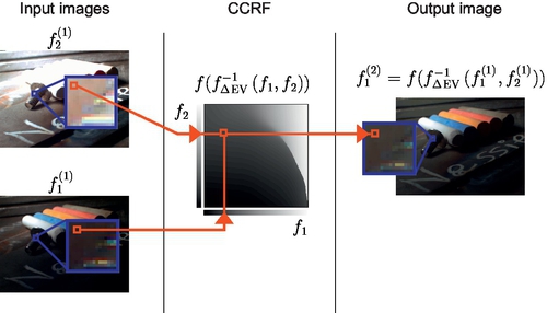
 , which returns a refined estimate of an ideal camera response to the scene being photographed. This virtual camera’s exposure setting is equal to the exposure of the lower-exposure image f1.
For efficient implementation, rather than computing at runtime or storing values of f−1(f1,f2), we can store f(f−1(f1,f2)). We call this the comparametric camera response function (CCRF). It is the comparametric inverse camera response function evaluated via (or “imaged” through, because we are in effect using a virtual camera) the camera response function f. This means at runtime we require N(N − 1)/2 recursive lookups, and we can perform all pairwise comparisons at each level in parallel, where a level is a row in Fig. 1.20.
The reason we can use the same CCRF throughout is because each virtual comparametric camera f ° f−1 returns an exposure that is at the same exposure point as the less exposed of the two input images (recall that we set k1 = 1), so Δev between images remains constant at each subsequent level.
In comparison with Fig. 3 in Mann and Mann (2001), wherein the objective is to recover the camera response function and its inverse, in this case we are using a similar hierarchical structure to instead combine information from multiple source images to create a single composite image.
The memory required to store the entire pyramid, including the source images, is N(N + 1) times the amount of memory needed to store a single uncompressed source image with floating-point pixels. Multichannel estimation (eg, for color images) can be done by use of separate response functions for each channel, at a cost in compute operations and memory storage that is proportional to the number of channels.
Alternative graph topology
Other connection topologies are possible — for example, we can trade memory usage for speed by compositing using the following form for the case N = 4 :
in which case we perform only three lookups at runtime, instead of six with the previous structure. However, we must store twice as much lookup information in memory: for ![]() as before, and for
as before, and for ![]() , because the results of the inner expressions are no longer Δev apart, but instead are twice as far apart in exposure value, 2Δev, as shown in Fig. 1.22. As a recursive relation for
, because the results of the inner expressions are no longer Δev apart, but instead are twice as far apart in exposure value, 2Δev, as shown in Fig. 1.22. As a recursive relation for ![]() we have
we have
where ![]() and i = 1,…,N/2j−1. The final output image is
and i = 1,…,N/2j−1. The final output image is ![]() , and
, and ![]() is the ith input image. This form requires N − 1 lookups. In general, by combining this approach with the previous graph structure, we can see that comparametric image composition can always be done in O(N) lookups
is the ith input image. This form requires N − 1 lookups. In general, by combining this approach with the previous graph structure, we can see that comparametric image composition can always be done in O(N) lookups ![]() .
.

The alternative form described so far is only a single option of many possible configurations. For example, use of multiple LUTs provides less locality of reference, causing cache misses in the memory hierarchy, and uses more memory. In a memory-constrained environment, or one in which memory access is slow, we could use a single LUT while still using this alternate topology, as in
This comes at the expense of our performing more arithmetic operations per comparametric lookup.
Constructing the CCRF
To create a CCRF f ° f−1(f1,f2,…,fN), the ingredients required are a camera response function f(q) and an algorithm for creating an estimate ![]() of photoquantity by combining multiple measurements. Once these have been selected, f ° f−1 is the camera response evaluated at the output of the joint estimator, and is a function of two or more tonal inputs fi.
of photoquantity by combining multiple measurements. Once these have been selected, f ° f−1 is the camera response evaluated at the output of the joint estimator, and is a function of two or more tonal inputs fi.
To create a LUT means sampling through the possible tonal values, so, for example, to create a 1024 × 1024 LUT we could execute our ![]() estimation algorithm for all combinations of
estimation algorithm for all combinations of ![]() and store the result of
and store the result of ![]() in a matrix indexed by [1023f1,1023f2], assuming zero-based array indexing. Intermediate values may be estimated by linear or other interpolation.
in a matrix indexed by [1023f1,1023f2], assuming zero-based array indexing. Intermediate values may be estimated by linear or other interpolation.
Incremental updates
In the common situation that there is a single camera capturing images in sequence, we can easily perform updates of the final composited image incrementally, using partial updates, by only updating the buffers dependent on the new input.
1.8.1 Example Joint Estimator
In this section we describe a simple joint photoquantity estimator, using nonlinear optimization to compute a CCRF. This method executes in real time for HDR video, using pairwise comparametric image compositing. Examples of the results of this estimator can be seen in Figs. 1.20 and 1.22.
1.8.1.1 Bayesian probabilistic model for the CCRF
In this section we propose a simple method for estimating a CCRF. First, we select a comparametric model, which determines the analytical form of the camera response function. As an example, we illustrate our compositing approach using the “preferred saturation” camera model (Mann, 2001), for which an analytical is known and can be verified by use of the approach in the previous section.
The next step is to determine the model parameters, as in Fig. 1.23; however, any camera model with good empirical fit may be used with this method.

 function, and color inverted, to show finer variation. The best results for comparametric compositing are found when the camera response function model parameters are optimized against a range of k values. Here k1 = 1 and k2 = 8, k3 = 64, and k4 = 512, which implies that for comparametric image compositing we would use ΔEV = 3.
Let scalars f1 and f2 form a Wyckoff set from a camera with zero-mean Gaussian noise, and let random variables Xi = fi − f(kiq),i ∈{1,2} be the difference between the observation and the model, with k1 = 1 and k2 = k.
We can estimate the variances of Xi can be estimated between exposures by calculating the interquartile range along each column (for X1) and row (for X2) of the comparagram with the Δev of interest (ie, using the “fatness” of the comparagram). A robust statistical formula, based on the quartiles of the normal distribution, gives ![]() , which can be stored in two one-dimensional vectors.
, which can be stored in two one-dimensional vectors.
Discontinuities in ![]() with respect to fi can be mitigated by Gaussian blurring of the sample statistics, as shown in Fig. 1.24. Using interpolation between samples of the standard deviation, and extrapolation beyond the first and last samples, we can estimate for any value of f1 or f2 the corresponding constant
with respect to fi can be mitigated by Gaussian blurring of the sample statistics, as shown in Fig. 1.24. Using interpolation between samples of the standard deviation, and extrapolation beyond the first and last samples, we can estimate for any value of f1 or f2 the corresponding constant ![]() or
or ![]() .
.

The probability of ![]() , given f1 and f2, is
, given f1 and f2, is

For simplicity, we choose a uniform prior, which gives us ![]() . Using Xi, we have
. Using Xi, we have
To maximize ![]() with respect to q, we remove constant factors and equivalently minimize
with respect to q, we remove constant factors and equivalently minimize ![]() . Then the optimal value of q, given f1 and f2, is
. Then the optimal value of q, given f1 and f2, is
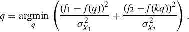
In practice, good estimates of optimal q values can be found with use of, for example, the Levenberg-Marquardt algorithm.
1.8.2 Discussion Regarding Compositing via the CCRF
Use of direct computation for nonlinear iterative methods as in Pal et al. (2004) is not feasible for real-time HDR video, because the time required to converge to a solution on a per-pixel basis is too long.
For our simplistic probabilistic model given in Section 1.8.1, it takes more than 1 min (approximately 65 s) to compute each output frame with a single processor. With the method proposed in Section 1.8, the multicore speedup is more than 2500 times for CPU-based computation, and 3800 times for graphics processing unit (GPU)-based computation (versus CPU), as shown in Table 1.3.
Table 1.3
Performance of Pairwise Composition Versus Direct Calculation of a Composite HDR Image on Four Input LDR Images
| Method | ||||
| Direct Calculation | CCRF, Full Update | CCRF, Incremental | ||
| Platform | Speed (output frames per second) | Speedup | ||
| CPU (serial) | 0.0154 | 51 | 78 | 5065 times |
| CPU (threaded) | 0.103 | 191 | 265 | 2573 times |
| GPU | – | 272 | 398 | – |

The selection of the size of the LUT depends on the range of exposures for which it is used. It was found empirically that 1024 × 1024 samples of a CCRF is enough for the practical dynamic range of our typical setups. Further increases in the size of the LUT resulted in no noticeable improvement in output video quality.
Because GPUs implement floating-point texture lookup with linear interpolation in hardware, and can execute highly parallelized code, the GPU execution would seem to be a natural application of general-purpose GPU computation. However, for this application much of the time is spent waiting for data transfer between the host and the GPU — the pairwise partial update is useful in this context because we can reuse partial results from the previous estimate, and transfer only the new data.
1.8.3 Review of Analytical Comparametric Equations
In this section have we developed the general solution to any comparametric problem. This solution converts the comparametric system from a functional equation to a separable ordinary differential equation. The solution to this differential equation can then be used to perform image compositing based on photoquantity estimation.
We have further illustrated comparametric compositing as a novel computational method that uses multidimensional LUTs, recursively if necessary, to estimate HDR output from LDR inputs. The runtime cost is fixed irrespective of the algorithm implemented if it can be expressed as a comparametric lookup. Pairwise estimation decouples the specific compositing algorithm from runtime, enabling a flexible architecture for real-time applications, such as HDR video, that require fast computation. Our experiments show that we approach a data transfer barrier rather than a compute-time limit. We demonstrated a speedup of three orders of magnitude for nonlinear optimization–based photoquantity estimation.
1.9 Efficient Implementation of HDR Reconstruction via CCRF Compression
High-quality HDR typically requires large computational and memory requirements. We seek to provide a system for efficient real-time computation of HDR reconstruction from multiple LDR samples, using very limited memory. The result translates into hardware such as field-programmable gate array (FPGA) chips that can fit within eyeglass frames or other miniature devices.
The CCRF enables an HDR compositing method that performs a pairwise estimate by taking two pixel values pi and pj at an exposure difference of Δev and outputs ![]() , the photoquantigraphic quantity (Ali and Mann, 2012). The CCRF results can be stored in a LUT. The LUT contains N × N elements of precomputed CCRF results on pairs of discretized pi and pj values. The benefit of the use of a CCRF is that the final estimate of photoquantity can incorporate multiple samples at different exposures to determine a single estimate of the photoquantity at each pixel.
, the photoquantigraphic quantity (Ali and Mann, 2012). The CCRF results can be stored in a LUT. The LUT contains N × N elements of precomputed CCRF results on pairs of discretized pi and pj values. The benefit of the use of a CCRF is that the final estimate of photoquantity can incorporate multiple samples at different exposures to determine a single estimate of the photoquantity at each pixel.
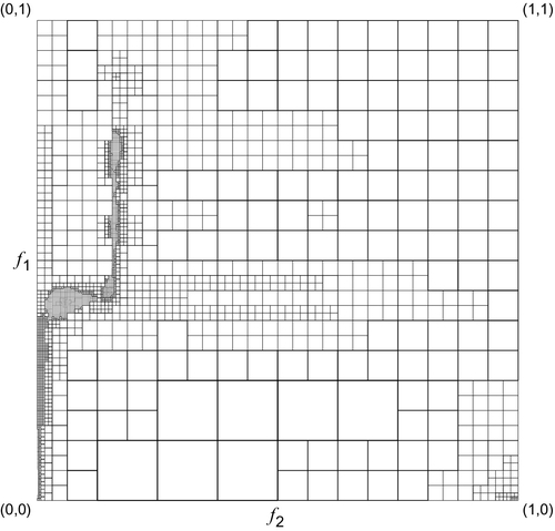
Quadtree representation
The CCRF LUT can be represented in a tree structure. For N × N elements, we can generate a quadtree (a parent node in a such tree contains four child nodes) to fully represent the CCRF LUT. Such a quadtree is a complete tree with ![]() or
or ![]() levels.
levels.
One method of generating such a tree is to recursively divide a unit square into four quadrants (four smaller but equally sized squares). We can visualize the center of a divided unit square as the parent node of the four quadrants. The center of each quadrant is considered a child node. Such a process is performed recursively in each quadrant until the root unit square is divided into N × N equally sized squares. The bottom nodes of the quadtree are the leaves of the tree, each of which stores the CCRF lookup value of the corresponding pixel pair (pi, pj).
Reducing the quadtree
Storing the leaves of the complete quadtree representation of the CCRF costs as much space as the CCRF LUT itself. To reduce the number of elements needed for storage, we proceed to interpolate the CCRF value ![]() of a specific pair (pi, pj) on the basis of its neighbor CCRF lookups. The value
of a specific pair (pi, pj) on the basis of its neighbor CCRF lookups. The value ![]() interpolated on the basis of its neighbors is compared against the actual CCRF lookup value pi,j, which gives ei,j, the error per lookup entry:
interpolated on the basis of its neighbors is compared against the actual CCRF lookup value pi,j, which gives ei,j, the error per lookup entry:
We accept the approximated result if ei,j is within a fraction of ![]() as the error threshold eth:
as the error threshold eth:
where α is the fraction constant and D is the bit depth of the pixel value. We define the neighbor CCRF points as the four corner CCRF points of the square. We interpolate all CCRF (pi, pj) within the same square on the basis of these four corner values. We denote ![]() as the indicator function of unsatisfied error condition:
as the indicator function of unsatisfied error condition:

We divide the square into four quadrants if
The purpose of the division is to obtain new corner values that are closer to the point. The closer corner values to the point for interpolation may yield lower ei,j as the CCRF LUT generally varies smoothly over a continuous and wide range of pi and pj values. Therefore, we expect that the density of the divisions corresponds to the local gradient of the CCRF LUT: the higher the local gradient, the more recursive divisions are required to bring corners closer to the point, whereas the points formed of a large and smooth region of the CCRF with low local gradient share the same corners.
Error weighting and tree depth criteria
The error of the interpolation against the original lookup value of the input pair (pi, pj) should be within eth. This error is affected by the interpolation method. Empirically, we find that bilinear interpolation works better than quartic interpolation in terms of minimizing the number of lookup points while satisfying the error constraint.
Statistically, we observe that the most frequently accessed CCRF values lie along the comparagram, as shown in Fig. 1.25. Therefore, higher precision on interpolation may not be necessary for CCRF lookup points that are distant from the comparagram. This suggests that the error constraint for the pair (pi, pj) should vary depending on its likelihood of occurrence. To further compress the CCRF LUT, we can scale ei,j by the number of observed occurrences of the pair (pi, pj). This information is obtained through the construction of the comparagram. For each entry of the CCRF lookup, we weight the interpolation error by directly multiplying it by the occurrence count observed on the comparagram:
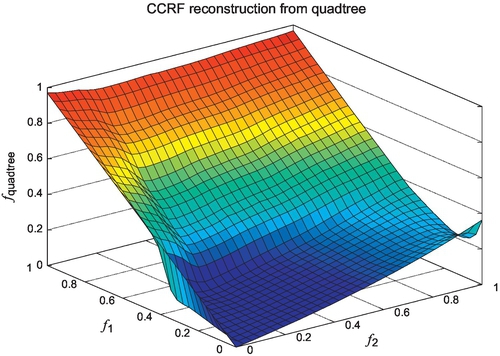
where Bi,j is the count of the number of occurrences on the comparagram entry of (pi, pj). The result with the weighted errors also favors bilinear interpolation over quartic interpolation in terms of minimizing the number of entries of the CCRF for storage, as shown in Fig. 1.26. Reconstruction of the original CCRF from this quadtree is shown in Fig. 1.27, with the corresponding error shown in Fig. 1.28.


The CCRF LUT we use has 1024 entries for pi and 1024 entries for pj. Therefore, there is no point in constructing a tree that has a depth of more than ![]() . We may constrain the depth of the tree to fewer than 10 levels as long as the error constraint is met. This affects the resulting number of entries in the CCRF quadtree, as well as the number of iterations required to find a leaf node.
. We may constrain the depth of the tree to fewer than 10 levels as long as the error constraint is met. This affects the resulting number of entries in the CCRF quadtree, as well as the number of iterations required to find a leaf node.
Corner value access
Each node of the quadtree is the center point of the square that contains it. To access the corner values of a leaf node, we can perform a recursive comparison of pair (pi, pj) with (px, py) of the nonleaf nodes in the tree until a leaf node has been reached, seen in Algorithm 1. The leaf nodes contain memory addresses of the corresponding corner values. The corner values of a leaf node are stored in the memory for retrieval.
1.9.1 Implementation
The algorithm can be implemented efficiently on a medium-sized FPGA. Given a finalized quadtree data structure, a system can be generated with software. The four corner values are stored in ROMs implemented with on-chip block RAM, and then selected by multiplexer chains based on the inputs f1 and f2. An arithmetic circuit that follows can then calculate the result on the basis of bilinear interpolation. Thus, as shown in Fig. 1.29, the system consists of two major parts: an addressing circuit and an interpolation circuit.

Because the size of the quadtree can grow to 10 levels, a C program is written to generate the implementation of the two circuits in Verilog hardware description language. Given a compressed data structure, this program generates four ROM initialization files and a circuit that retrieves corner values stored in the ROMs based on the inputs.
1.9.1.1 Addressing circuit
Each of the quadtree leaves needs a unique address. This address is used to retrieve the corresponding corner values from ROMs. As shown in Fig. 1.30, the circuit outputs the address by comparing f1 and f2 with constant boundary values, in the same way as we traverse the quadtree. The main function of the boundary comparator is to send the controlling signal to traverse the multiplexer tree, on the basis of the given input pair. At each level, it compares the input values with the prestored center coordinate values, and determines which branch (if exits) it should take next. Otherwise, the current node is a quadtree leaf and a valid address will be selected.

The algorithm generates the circuit by traversing the quadtree. Because a new unique address is needed for every leaf being visited, a global counter is used to determine the addresses. The width of the circuit data path is then determined with the last address generated (ie, the maximum address).

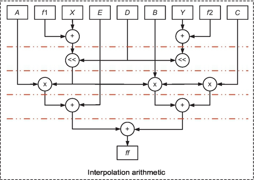
1.9.1.2 Interpolation circuit
The circuit takes the address and uses it to look up values that are prestored in the block RAM. These values can be used to perform an arithmetic operation (as shown in Fig. 1.31) for bilinear interpolation. To maintain high throughput, the intermediate stages are pipelined with use of registers.
1.9.2 Compression Performance
The compressed CCRF LUT requires storage of all corner values per pair (pi, pj) for interpolation. Without any compression, this method would require as many as four times the storage space because of redundancies of identical CCRF values shared between adjacent lookups. However, the compression is able to reduce the number of lookup entries by a factor greater than four times. This compression factor depends on the selection of α.
We wrote the compression in the C programming language to output the compressed CCRF LUT. In Table 1.4, we list the minimum compression factor and the expected error over the entire CCRF range, for four selections of α.
Table 1.4
Quadtree Properties Depending on the Choice of α
| Maximum Depth = 8 | α = 1 | α = 1/2 | α = 1/4 | α = 1/16 |
| Number of entries | 3315 | 4828 | 6508 | 10,807 |
| Compression factor | 79.1 | 54.2 | 161.1 | 97.0 |
| Mean depth | 5.8 | 6.2 | 6.6 | 7.4 |
| Expected depth | 7.7 | 7.8 | 7.8 | 7.9 |
| Error constraint | 0.0039 | 0.0019 | 0.00098 | 0.00024 |
| Expected error | 0.00042 | 0.00038 | 0.00036 | 0.00035 |

Notes: The compression factor is calculated on the basis of the number of CCRF lookup entries required divided by the number of the entries after compression. The CCRF without compression contains 106 floating-point entries.
The minimum compression factor summarizes the amount of compression achieved by taking the ratio of the total number of entries in the CCRF LUT to the number in the compressed one:
The constant 4 is the upper bound of the maximum redundancy of the corner value storage that overlaps with adjacent CCRF lookup points.
1.9.2.1 Hardware resource usage
For resource estimation without consideration of optimization effort performed by the CAD tool, we have

The actual number of resources needed to implement the system is much less (almost halved) than what we expected. The detailed data gathered from both expectation (using counters) and the CAD outputs are summarized in Table 1.5.
Table 1.5
The Resource Usage of the Implementation on a Kintex 7 (Xilinx XC7K325T) FPGA
| Depth = 4 | Depth = 6 | Depth = 8 | Depth = 10 | |
| Expected slice usage | 63 | 633 | 3315 | 21,207 |
| Portion used (%) | 0.0309 | 0.31 | 1.6 | 10 |
| Actual slice usage | 2 | 119 | 737 | 11,101 |
| Portion used (%) | 9.8 × 10⁻⁴ | 0.058 | 0.36 | 5.5 |

Notes: The total number of logic slices used in this FPGA is 203,800. The difference between the expected and actual usage is due to the optimization present in the synthesis process, enabling more efficient use of resources.
1.9.3 Conclusion
This section presented an architecture for accurate HDR imaging that is amenable for implementation on highly memory constrained low-power FPGA platforms. Construction of the compositing function is performed by nonlinear optimization of a Bayesian formulation of the compositing problem, where the selected prior creates an accurate estimator that is smooth for robustness and enhanced compression. The estimator is solved over a regular grid in the unit square, forming a two-dimensional LUT. Implementation of this solution on an FPGA then relies on the compression of the LUT into a quadtree form that allows random access, and uses bilinear interpolation to approximate values for intermediate points. This form allows selective control over error bounds, depending on the expected use of the table, which is easily obtained for a particular sensor. This results in compression of more than 60 times relative to the original LUT, with visually indistinguishable results.