
Creating HDR Video Using Retargetting
F. Banterle*; J. Unger† * CNR-ISTI, Pisa, Italy
† Linköping University, Linköping, Sweden
Abstract
Capturing HDR videos is still a challenging task because HDR camera systems are either very costly (commercial systems) or have not matured enough to reach consumer markets (research prototypes). Recently, unofficial firmware for cameras has started to appear, and the firmware allows for reprogramming of the system to capture footage with an extended dynamic range. The dynamic range that can be captured in a single shot, however, is still limited and does not fully cover the dynamic range found in high-contrast scenes. There is, therefore, a need for low-cost techniques that allow for HDR-video capture using off-the-shelf equipment. This chapter describes methods for enhancing the standard dynamic range using previously captured HDR photographs of the same scene.
Keywords
High dynamic range imaging; High dynamic range video; Standard dynamic range enhancement; Standard dynamic range video
1 Introduction
Capture of HDR still images is now well known and from many aspects, a solved problem; see [1, 2] for an overview. However, HDR video capture still remains a challenge. There are a number of professional systems, such as the Arri Alexa XT and the Red Epic Dragon, with an extended dynamic range of up to 14–16.5 f-stops, and research prototypes [3, 4], with a dynamic range of up to 20–24 f-stops. However, these camera systems either still have a limited dynamic range and are very costly (commercial systems), or have not matured enough to reach consumer markets (research prototypes). An important area is to develop methods that allow users to capture HDR video using low cost off-the-shelf technology, such as ordinary video cameras and standard DSLR cameras.
This chapter gives an overview of two practical methods for generating HDR videos by retargeting information from a set of sparsely captured HDR images or panoramas onto a standard dynamic range (SDR) videos, captured in the same scene. The first method by Bhat et al. [5] aims to register and fuse a dense SDR video with sparse HDR photographs in static scenes with moving cameras by exploiting computer vision algorithms for registration. The second method by Banterle et al. [6] solves the problem in the case of a static SDR video camera (a static background) and a dynamic scene, such as people or objects moving in the scene. The method is carried out as a completely automatic postprocessing phase, i.e., after the input footage has been captured. The two techniques are useful in different application scenarios: from the acquisition of medium-to-high quality videos, to the typical case of webcams, where a satisfying trade-off in exposure between the subject in foreground and the usually bright background is difficult (if not impossible) to find.
2 Background in HDR Video and Image Retargeting
The goal of the two methods described in this chapter is to create HDR videos by fusing or retargeting image data captured as dense SDR video footage, and sparse image data captured using HDR imaging techniques. We start this chapter by giving an overview of methods for HDR capture, and an overview of related work in, and the concept of, image retargeting.
2.1 HDR Video Capture
The dynamic range of a camera refers to the ratio between the highest intensity and the lowest intensity and the sensor can accurately capture within the same frame. The lowest intensity is usually defined by an acceptable signal-to-noise ratio. Here, we use the term HDR image to mean an image, which covers the full dynamic range of the scene. This means that no pixels are saturated and that all pixels can be trusted as a measurement of the scene radiance with a linear response to the number of photons detected. Each pixel and color channel in an HDR image is usually represented as a 32- or 16-bit precision floating point number, instead of an 8-bit integer as in traditional images.
The typical dynamic range exhibited by current high-end and consumer camera systems is in the order of 10,000:1. This should be compared to the dynamic range found in real scenes, which in many cases extends beyond 1,000,000:1, from direct light sources to shadows. This is significantly more than the dynamic range of most camera systems can capture. Fig. 1 shows an example of HDR image as four tone mapped exposures. The four images are generated three f-stops apart from the original HDR image by linear scaling of the input pixels, gamma mapping, and finally quantization of the floating point data into 8 bits per pixel and (R,G,B) color channel.

In the professional segment there are cameras, e.g., the Red Epic Dragon and Arri Alexa XT, with an extended dynamic range of up to 16 f-stops, corresponding to a dynamic range in the order of 100,000:1. There are also image sensors with a logarithmic response that can capture a significantly higher dynamic range. However, these sensors are, in general, not suitable for high-quality imaging applications because they usually have a comparably low resolution and suffer from image noise in darker regions. To enable capture of images with a dynamic range larger than the approximately 16 f-stops offered by high-end cameras, it is currently necessary to perform some form of multiplexing. The multiplexing can be carried out in different ways, e.g., in the temporal domain by capturing different exposures, in the radiometric domain by using multiple image sensors, or in the spatial domain by inserting filters that vary the transmittance of light on a per-pixel level.
The traditional approach for capturing HDR images is to capture a set of different exposures covering the dynamic range of the scene and merge them into the final HDR image [7–9]. This approach is often referred to as exposure bracketing, and many modern cameras can be set to do this automatically. The main drawback with this method is that it requires both the camera and the scene to be kept static during capture, due to the fact that a set of images with different exposure settings needs to be captured. Unger et al. [10, 11] developed an HDR video camera system where the time disparity between the different exposures was minimized by capturing four different exposures back-to-back for each row on the sensor in a rolling shutter fashion, instead of waiting for the entire image to be captured. To extend the dynamic range further, they also A/D converted each pixel value twice with different amplification of the analog pixel readout, i.e., the images were captured with two different ISO values simultaneously. There are also algorithms for compensating for the misalignments introduced by camera motion or dynamic objects [12]. However, these methods are, in most cases, not fully robust and may still lead to artifacts.
Another approach is to use multiple, synchronized camera sensors imaging the scene through the same optical system. This technique is suitable for capture of HDR video, because the sensors capture all exposures at the same time. Robustness to dynamic scenes and correct motion blur can be ensured by using a common exposure time. The exposures captured by the sensors can be varied by inserting different filters. For example, Kronander et al. [4, 13] proposed natural density (ND) filters in front of four different sensors built into the same camera setup. Similarly, Froehlich et al. [14] used two Arri Alexa digital film cameras capturing the scene through zero baseline stereo setup. However, the use of ND filters in the optical path leads to a waste of light, i.e., longer exposure times. This is because a lot of the incident radiance is simply filtered out. To avoid this issue, Tocci et al. [3] introduced a multisensor setup with three sensors without ND-filters. Instead of using ND filters, they show how the beam-splitters themselves can be used to reflect different amounts of the incident light onto the different sensors.
Another possibility is to trade spatial resolution against dynamic range by using a sensor where the response varies between pixels. The advantage is that all exposures are captured at the same time and with the same exposure time. Spatially varying exposures [15] can be achieved by placing a filter mask with different transmittance on top of the sensor. This idea is similar to color imaging using a single sensor using, e.g., a Bayer pattern color filter array, but with the difference that in addition to the (R,G,B) color filters, there are also ND filters distributed over the sensor. Another approach is to let the per-pixel gain, or ISO, vary between groups of pixels over the sensor; see for example Hajisharif et al.’s work [16]. This functionality is currently available for off-the-shelf Canon cameras running the Magic Lantern firmware1 as further described in Chapter 4. The disadvantage of the spatial multiplexing approach is the trade-off between resolution and achievable dynamic range, as too many different exposures may lead to a lower resolution in the reconstructed HDR image.
2.2 Image Retargeting
Image retargeting, in the sense of improving existing images or videos with higher quality content, is a very broad research topic in computer graphics and imaging. Retargeting can happen for different image/video frame attributes, such as image resolution, color information, temporal resolution, and dynamic range; see [17] for an overview. In this section, we want to highlight a few works which are closely related to the problem of enhancing SDR content using HDR reference photographs.
Wang et al. [18] proposed a method for increasing the dynamic range and transferring the detail from a source LDR image into a target LDR image. While the dynamic range expansion is automatic by fitting Gaussian profiles around overexposed regions, the details transfer part is manual. In this case, a user needs to transfer high-frequency details from a well-exposed area (or another image) to an overexposed or an underexposed area using a tool similar to the healing tool of Adobe Photoshop.2 Although this method produces high-quality results, it cannot be applied to videos because the user interaction is extremely heavy.
Regarding retargeting videos resolution, Ancuti [19] proposed a simple technique to transfer detail from a high-resolution image to the video. In their work, SIFT features [20] are extracted from both high-resolution images and low-resolution video frames, and then they are matched. Matched patches in the high-resolution photographs are then copied onto the low-resolution frames, obtaining a high-resolution output video. Similarly, Gupta [21] extended this concept by designing a framework based on high-quality optical flow and image-based rendering. This can be implemented in video-cameras that can acquire both photographs and videos. However, both these works do not handle HDR information during the retargeting of the input SDR video.
3 Dynamic Camera and Static Scene
SDR videos can be enhanced when the scene is static, but the camera moves using Bhat et al.’s system [5]. This system, depicted in Fig. 2, requires as input a few HDR photographs of a static scene and an SDR video of the scene, and it outputs an enhanced video where the HDR information from photographs is transferred onto the SDR video.

The system has two main components:
• a geometry estimation component for estimating depths and correspondences;
• an image-based renderer for video reconstruction.
3.1 Geometry Estimation
As the first step, the system applies a structure-from-motion (SfM) algorithm [22] in order to compute a sparse point cloud, including projection matrices for each photograph and video frame, and a list of the viewpoints from which each scene point is visible (see Fig. 3).

Then, a modified multiview stereo (MVS) algorithm [23] is employed for computing depth maps for each video frame and HDR photograph. This MVS algorithm segments the image based on colors, and it then computes disparity for each segment by constructing a pair-wise Markov random field (MRF) for each image. Bhat et al. extended it to take into account heterogeneous datasets (photographs and frames), wide range of disparity planes, and 3D points in the point cloud from SfM to improve depth estimation. An example of generated depth maps is shown in Fig. 4.

3.2 Video Reconstruction
The correspondence found using SfM and the MVS modified algorithm (see previous section) are then used to reconstruct an HDR video, using the HDR information of the photographs while preserving the temporal dynamics of the SDR input video.
An approach to solve this problem is to use the classic view interpolation approach [24, 25]. However, images warped with view interpolation can suffer in ghosting artifacts and loss of high-frequency details. To overcome these issues, the authors proposed to formulate the reconstruction problem as a labeling problem in a MRF network. The goal is to assign to each pixel p of the ith video frame, Vi, a label, L(P), which indicates the candidate HDR photograph that should contribute to the final result. This candidate is chosen among the N nearest HDR photographs to Vi that are reprojected from the viewpoint of Vi. This leads to the following cost function:

where CD is the data cost function encouraging video pixels to be reconstructed from photographs with similar color and depth, CS is the smoothness term similar to the one by Kwatra et al. [26], n is a set of all eight-connected neighbors in Vi, p and q are neighboring pixels defined by N, and λ is a trade-off between CD and CS. Eq. (1) is solved using a graph-cut optimization [27] obtaining a reconstructed video R.
The output video computed in the MRF reconstruction may suffer from artifacts such as lack of rich temporal variations, seams in the frame (i.e., different HDR photographs used in different areas of the frame), holes (due to missing portions of the scene not seen in any of the HDR photographs). To solve these issues, a gradient domain composition is employed by using motion compensated temporal gradients, Gt, from the input SDR video, and spatial gradients, Gx and Gy, from R. Note that in the case of holes in R; temporal gradients from the original videos are copied and matched using color transfer [28]. The final enhanced video, E, is created by solving an over constrained linear system defined by the following constraints in a gradient domain fashion as:
where (u, v) is a motion vector linking the pixel at (x, y, t) to its corresponding one in the frame t + 1. Eq. (4) can be solved with a conjugate gradient solver [29]. Note that Eq. (4) requires to have all the videos to be in memory. If this is not the case, the linear system can be solved for slabs of 20–30 frames using Dirichlet boundary conditions.
3.3 Discussion
Bhat et al. successfully tested for retargeting SDR videos (see Fig. 5). Furthermore, this system is extremely flexible, and it can be employed for different tasks such as super-resolution, exposure correction, video editing, camera shake removal, and object removal.

One main drawback of the system is still the presence of some image artifacts in the output video, due to the errors of some computer vision algorithms used in the pipeline, such as oversegmentation in the MVS, and imprecise projection matrices from SfM.
Timing Bhat et al. implemented the system in C++ without optimizations, reporting on average around 5 minutes for enhancing an 853 × 480 frame on an unspecified 2007 machine.
4 Static Camera and Dynamic Scene
When the camera is static and the scene is dynamic, Banterle et al.’s algorithm [6] can be employed. This method, depicted in Fig. 6, requires as input a single HDR photograph of the background and an SDR video of the scene taken using a static camera, and it outputs an enhanced video where the HDR information from HDR background photograph is transferred onto the SDR video. Note that the exposure of the input SDR video footage is manually set in order to have actors or important moving objects in the scene well exposed.

4.1 The Blending Algorithm
The HDR background photograph and the SDR video are blended together in a straightforward way. As the first step, the SDR video footage is linearized applying the inverse camera response function of the SDR video-camera. After linearization, the SDR video is scaled by the capturing shutter speed, obtaining a normalized SDR video with absolute values. Linearization and scaling are important in order to match intensities and colors with the HDR background photograph. In fact, this makes it possible to use less computationally expensive techniques for the blending stage.
At this point, the HDR image and the normalized and scaled SDR frame are linearly blended in the logarithm domain, using a selection mask M, which classifies background and actors. The blending is applied in the logarithmic domain to avoid seams at the mask’s boundaries. Then, the blended image is exponentiated to obtain the final radiance map. This straightforward blend is enough to obtain no seams or other kind of artifacts. Other techniques, as Laplacian pyramids [30] and Gradient Domain editing [31–33], produce similar results of the linear blending at higher computational costs. Furthermore, in some cases, the colors are slightly shifted; see Fig. 7 for a comparison.

4.2 The Classification Mask
The classification mask, M, is computed using thresholding on overexposed and underexposed pixel values on the luminance channel for each frame of the video. Authors found that 0.95 and 0.05 are, respectively, good threshold for overexposed and underexposed thresholds; using normalized RGB values. Thresholding can produce groups of single pixels in the image, which is typically to be considered as noise. Therefore, morphological operators, erosion followed by dilation, need to be applied. Typically, 3–5 iterations are enough for obtaining high-quality results on full HD content (1920 × 1080). Finally, the mask is cross bilateral filtered with the original SDR luminance frame using a fast bilateral filter [34, 35] (σs = 16 and σr = 0.1 for full HD content) in order to smoothly extend the classification to strong edges. Fig. 8 shows an example of the different steps for calculating the mask.

4.3 Discussion
This algorithm has a very simple acquisition step, and the processing is fully automatic. Therefore, it can be used for different setups, such as webcams and a medium/high-end cameras. Below, we give an overview of different use cases using input SDR videos of different quality.
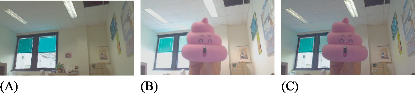
Webcams. Webcams are usually not able to find a trade-off exposure between the foreground subject and the background, especially during video calls. To test the method, Banterle et al. used a Logitech QuickCam Pro 9000, which captures videos with a 1280 × 720 resolution. The example in Fig. 9 shows the selection of the best exposure for the main subject, while background information is recovered during the blending. Fig. 9C shows that a convincing HDR can be obtained with this device, although part of the range is missing due the limitations of the camera.
Medium/High-End Cameras. Banterle et al. also evaluated the method using input SDR video from a Canon 550D, which is able to acquire videos at 1920 × 1080 resolution. The method can work in difficult lighting conditions. In the example shown in Fig. 10, a tone mapped version of the HDR background is shown in Fig. 10A. Fig. 10B shows a frame of the original SDR video, where most of the background and the sky are overexposed. Using the HDR background image, the enhanced video recovers the appearance of the sky and of several overexposed parts (see Fig. 10C).

A second example, Fig. 11, shows an indoor environment, where the light and part of the outdoor scene are lost. The enhanced video recovers this information. The colors in the frame enhanced are different from the ones in the SDR frame because the linearization process matches color curves between HDR background and SDR frame.

Timing. Authors reported on average less than 9 seconds for a 1920 × 1080 frame on an Intel Core 2 Duo at 2.33 GHz equipped with 3 GB of memory and Windows 7 using a MATLAB implementation.
5 Summary
This chapter presented two methods for augmenting SDR video sequences with HDR information in order to create HDR videos. The goal of the two methods is to fill in saturated regions in the SDR video frames by retargeting nonsaturated image data from a sparse set of HDR images. Table 1 shows a summary of the flexibility of the two approaches as compared to using an HDR video camera system as described in Section 2.
Table 1
A comparison between using specialized HDR video cameras and the two retargeting methods described in this chapter
| Capture type | Camera movement | Scene type |
| Bhat et al. [5] | Dynamic | Static |
| Banterle et al. [6] | Static | Dynamic |
| HDR native capture | Dynamic | Dynamic |
The HDR video cameras are naturally better equipped to capture fully dynamic HDR videos. However, current HDR video cameras are either research prototypes or not able to capture more than up to around 16 f-stops. The first method, by Bhat et al. [5], uses SfM techniques to register the SDR video and the sparsely captured HDR images to the same frame of reference and replaces pixels that are saturated in the SDR video with information from the HDR images. However, the technique may fail in regions where there is no overlap between the SDR video and the HDR images. The second method, by Banterle et al. [6], works for dynamic scenes, but it assumes that the camera is static, i.e., no camera movements. Under the assumption that moving people and/or objects are well exposed in the SDR video, this method replaces saturated pixel values in the background in order to generate an HDR video covering the full dynamic range of the scene. In conclusion, if the HDR images used to augment the SDR footage are captured carefully, the retargeting methods described in this chapter are a good option for generating HDR videos.