
Ghosting in HDR Video
A.O. Akyüz*; O.T. Tursun†; J. Hasić-Telalović‡; K. Karađuzović-Hadžiabdić‡ * Middle East Technical University, Ankara, Turkey
† Max Planck Institute for Informatics, Saarland, Germany
‡ International University of Sarajevo, Sarajevo, Bosnia and Herzegovina
Abstract
HDR video capture is a very important problem, the solution of which can facilitate the transition to an end-to-end HDR video pipeline. This problem is currently being tackled using various approaches. On the hardware front, there exist designs with a judicious combination of multiple off-the-shelf components such as lenses, mirrors, beam-splitters, and sensors, as well as designs that involve high dynamic range sensors. On the software front, many HDR video deghosting algorithms exist that enable creation of HDR videos from differently exposed successive frames. These algorithms need to deal with motion within the captured scene, as well as the motion of the capture device to produce artifact-free HDR videos. This chapter provides an overview of the most notable algorithms in both approaches, with an emphasis on HDR video deghosting algorithms. For further reading, we refer the interested readers to other excellent resources on this topic.
Keywords
High dynamic range; Motion compensation; Deghosting; Global alignment; Local alignment
1 Introduction
High-quality HDR videos can be captured in the following two ways: (1) by using dedicated video capture hardware that has improved dynamic range and (2) by using standard hardware to capture a set of frames with alternating exposures and then combining these frames for extending the dynamic range. We will call these two groups of techniques simultaneous and sequential HDR video capture methods.
Simultaneous HDR video capture typically entails the use of sensor elements with improved dynamic range. This method is usually employed by commercial products. However, it can also be performed by spatially varying the exposure of each sensor element, spatially varying the transmittance of neutral density filters placed in front of the sensor, or using a beam-splitting system to redirect the incoming light into multiple sensors, each set to a different exposure value. In this latter case, it becomes necessary to merge the output of the individual sensors to obtain an HDR frame.
Sequential HDR video capture, on the other hand, involves capturing of frames with alternating low and high exposures. This variation can be achieved by changing the exposure time, aperture size, or the sensitivity (ISO) of the camera between frames. In these techniques, each frame of the video is captured in low dynamic range (LDR), but has the potential to be converted to HDR by using the information present in the adjacent frames. These sequential techniques have recently become popular thanks to programmable digital cameras or third party software that allows capturing such alternating sequences. For example, Magic Lantern [3] is a software that furnishes most Canon DSLR cameras with this feature.
For both simultaneous and sequential systems, the merging of multiple exposures is motivated by the fact that each exposure contains details for different parts of the scene corresponding to different light levels. By merging this information, one can obtain an HDR frame that well represents a wider range of light levels of the captured scene.
However, the merging process may itself give rise to artifacts if the merged exposures are inconsistent with each other. Such inconsistencies may occur, for example, due to camera and object motion. In the case of camera motion, the exposures can be registered by global alignment techniques. However, this can still be problematic due to the parallax effect in which nearby objects are displaced more than the distant ones. In this case, a simple global alignment would not be sufficient. If the objects themselves are dynamic, this generates more complicated motion patterns, especially if this is combined with the camera motion. The field of HDR video deghosting typically deals with problems of both kinds.
2 Image Acquisition Model
In this section, we formalize the concept of creating an HDR image (or video frame) from multiple exposures. Here, we also introduce a terminology that we will use when describing the deghosting methods in more detail. Such a consistent terminology will allow focusing on the algorithmic differences rather than symbolic ones.
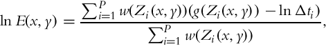
We assume that for frame i, each sensor element (x, y) is exposed to a radiance value E(x, y) for a duration of Δti seconds. This results in the total collected charge of E(x, y)Δti units. This collected charge passes through various transformations such as analog to digital conversion, quantization, gamma correction, and various custom transformations defined by the camera manufacturer. The net effect of these transformations is represented by using a function f, which is known as the camera response function [4]. Thus the relationship between the input irradiance and output pixel values, Zi(x, y), can be written as:
As the goal of HDR image and video generation is to recover the scene radiance values, it is necessary to estimate the (inverse) camera response function to reverse the above relationship:
However, due to limitations of the image sensor, not all pixels provide useful information about the scene. For example, it is impossible to estimate the correct radiance value for saturated (under- or overexposed) pixels. Furthermore, each pixel is a noisy measurement of the scene radiance. As a result, estimating the true radiance from a single exposure is generally not reliable. To address this problem, various solutions have been proposed. A simple and commonly used solution is to combine multiple exposures of the same scene captured simultaneously or in rapid succession.
Typically, multiple exposures are combined by assigning a weight to each of them based on the reliability of each exposure. First of all, if Zi(x, y) was clipped due to being under- or overexposed, this measurement does not represent the true scene radiance, hence its influence should be minimized. Second, the signal-to-noise ratio and the coarseness of quantization are generally not uniform across the valid range of the sensor. Therefore, both of these factors are taken into account to derive a final weighting function, w, that can be used to combine the sensor irradiances:
Here, for notational simplicity, we indicated the weighting function as to take a single input, which is the pixel value. However, it should be remembered that w may actually depend on various other factors such as the exposure time, camera response function, and the assumed noise model. We refer the reader to Granados et al. for a detailed review of different ways of setting the weighting function [5].
For color images, the typical practice is to treat each color channel independently to obtain ![]() ,
, ![]() , and
, and ![]() for red, green, and blue color channels, respectively. However, to avoid potential color casts, it may be desirable to use a combined value, such as luminance, in the computation of the weighting function [6].
for red, green, and blue color channels, respectively. However, to avoid potential color casts, it may be desirable to use a combined value, such as luminance, in the computation of the weighting function [6].
This simple formulation leads to blending artifacts if the corresponding pixels in different exposures belong to different parts of the scene. This could happen due to various factors, such as the movement of the camera, objects, and changes in illumination. To address this problem, Eq. (3) must be revised such that it allows us to combine pixels at different spatial coordinates. This may be accomplished by replacing (x, y) with (ui, vi) on the right-hand side of Eq. (3), where (ui, vi) represents the coordinates of a pixel in exposure i in some neighborhood of (x, y). Ideally, all (ui, vi) coordinates represent the same scene point in all exposures. In general, HDR image and video deghosting methods differ with respect to various strategies they employ to find these corresponding pixels.
3 HDR Image Deghosting Methods
As most HDR video deghosting methods are based on or inspired from HDR image deghosting methods, in this section we will summarize their main characteristics. For a detailed review of HDR image deghosting methods, we refer the reader to a survey paper by Tursun et al. [7].
A high-level taxonomy of HDR image deghosting methods is given in Fig. 1. According to this taxonomy, image deghosting methods are divided into four main categories as (1) global exposure registration, (2) moving object removal, (3) moving object selection, and (4) moving object registration.
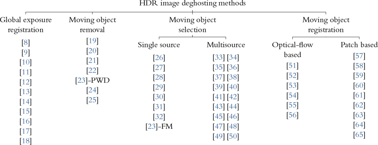
The first category only involves methods that perform global registration of the multiple exposures. While some of these techniques only handle translational misalignments such as Ward [10] and Aky![]() z [17], others can handle both rotational and translational misalignments such as [14]. In general, these techniques assume that the captured scene is static or the moving objects occupy small regions, as not to interfere with the registration process. However, as noted in Section 1, if the captured scene has multiple objects at different distances from the camera, global misalignments caused by pure camera motion may still be problematic due to the parallax effect.
z [17], others can handle both rotational and translational misalignments such as [14]. In general, these techniques assume that the captured scene is static or the moving objects occupy small regions, as not to interfere with the registration process. However, as noted in Section 1, if the captured scene has multiple objects at different distances from the camera, global misalignments caused by pure camera motion may still be problematic due to the parallax effect.
The second category involves methods that eliminate moving objects all together. In other words, they estimate the static background of the captured scene. A pioneering example of this group of algorithms is Khan et al. [19], which assumes that most pixels belong to static regions. By considering the similarity of pixels to each other in small spatiotemporal neighborhoods, the influence of dissimilar pixels (i.e., pixels belonging to moving objects) is minimized.
The third category, moving object selection, is comprised of deghosting methods that include moving objects in the output HDR image. Single-source methods may use only one reference exposure (e.g., the middle exposure) in all dynamic regions or they may choose a different source exposure for dynamic region based on the well-exposedness of the exposures. Multisource methods, on the other hand, try to combine as many exposures as possible that are consistent with each other in each dynamic region. For example, Oh et al. [42] postulate the HDR reconstruction problem as rank minimization of a matrix in which each column corresponds to an input exposure. By minimizing the rank of this matrix, the authors obtain pixels that are consistent with each other. Normally, this yields the static background of the captured scene. However, their method allows the user to choose a reference exposure which may contain moving objects of interest. The remaining exposures are then combined with this reference exposure based on how well they model the background.
The last category of HDR deghosting algorithms contains the most advanced methods in that they involve registering individual pixels across different exposures. The first subcategory is made up of optical flow based methods which work well when the motion is relatively small and there are a few occlusions (the tracked pixels do not get lost due to being hidden by another object). The second subcategory, on the other hand, describes each pixel by using a patch of varying sizes around that pixel and tries to find the best matching pixels by considering the similarity of their patches. In general, these methods appear to produce the highest quality HDR images with Sen et al. [62] being a pioneering example.
The large number of HDR image deghosting methods gave rise to various studies that evaluate their performance. Among these, both subjective and objective evaluations have been conducted. We refer the reader to Tursun et al. for a review of these methods [66].
4 HDR Video Capture Methods
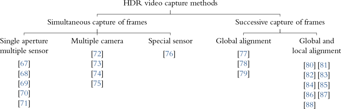
As discussed in the beginning of this chapter, there are various HDR video capture methods, termed simultaneous capture, that entirely avoid the deghosting problem. However, these methods require changes in the camera hardware and therefore cannot be readily used by most photographers and enthusiasts. These methods are discussed in this section. Alternatively, one can use existing digital cameras to capture the successive frames with different exposures, termed sequential capture. This results in a sequence of short and long exposures (sometimes alternation occurs between more than two exposures). In a post processing step, these exposures are registered using various techniques and then combined into HDR frames to form an HDR video. These techniques are divided into two groups based on whether they deal with ghosting at a global (Section 5) or local (Section 6) level. A taxonomy including both simultaneous and successive methods is given in Fig. 2.
4.1 Single Aperture Multiple Sensor Solutions
These groups of algorithms record the scene from a single aperture. The light that enters the aperture is then projected onto multiple sensors through a beam-splitting element. Each sensor is set to a different exposure value, which allows it to capture a different range of illumination. The sensor outputs are then combined to produce an HDR frame. This form of image generation is also called split-aperture imaging [2]. In general, this group of algorithms entirely avoids alignment and ghosting problems, as all sensors receive the same input.
A pioneering algorithm of this kind, in fact, utilizes a single sensor placed behind a transparency mask with multiple bands [89]. In other words, although there is a single sensor, different parts of the sensor receive different amounts of light depending on the transparency of the mask that is adjacent to it. The camera is designed as a panoramic camera, which rotates around its central axis. This allows the same scene point to be projected on different parts of the sensor with different exposures. As such, each scene point will be captured under multiple exposures. As the angular step size of the motor is known, one can compute the corresponding sensor positions of the same scene points, allowing them to be merged into a panoramic HDR image. This work does not propose a solution for dealing with potential changes in the scene during the capture process and therefore, it is suitable to capture only static scenes. A later work by the same authors extends this method to capture images at high frame rates, which are suitable to capture HDR videos, by using a beam-splitting mirror [67].
Wang and Raskar use a split-aperture camera to capture HDR videos [68]. The corner of a cube is used to generate a three-face pyramid, which transmits light toward three CCD sensors. Each sensor is adjacent to an ND filter with transmittances of 1, 0.5, and 0.25. The sensors are carefully aligned with respect to the pyramid such that the sensors are normal to the optical axis.
The beam-splitting approaches discussed earlier are wasteful of light in that they admit only a fraction of the light toward sensors. For example, if three-way beam-splitting is used, each sensor receives only one-third of the incident light. This light is further attenuated by the ND filters adjacent to the sensors. This reduction in light compels the photographer to use longer exposure times, which in turn may introduce problems such as thermal noise and motion blur. To address this problem, Tocci et al. propose a novel system that uses two beam-splitters which allow reusing the optical path to improve light efficiency [69]. Furthermore, they modify the HDR merging equation to consider the neighbors of a pixel rather than treating each pixel individually. This mitigates the cross-talk artifacts that may occur, for example, if a neighboring pixel is saturated, but the pixel itself not. Furthermore, it allows a smoother transition between pixels taken from different exposures.
The methods discussed earlier assume that sensors are perfectly aligned such that the same scene point is projected to the same locations in different sensors. However, this may be difficult to achieve in practice. Kronander et al. address this problem by assuming there exists an affine transform relating the coordinate system of each sensor to a virtual reference [70]. This transform is found in an offline stage by matching the corners of a checkerboard pattern. This method is later extended to capture HDR videos that perform demosaicking, denoising, alignment, and HDR assembly within a unified approach [71].
4.2 Multiple Camera Solutions
These group of algorithms utilize two or more cameras installed on a custom rig. Each camera captures the scene from its own viewpoint and with a different exposure time. The recorded frames must be registered prior to combining them to create HDR frames.
The first work that utilizes a multicamera solution was proposed by Ramachandra et al. [72]. In their system, the authors utilize a two-camera setup, whereby one camera is set to a short exposure time and the other to a long exposure time. As the longer exposed frames may be subject to motion-blur, the first step of their algorithm is deblurring of the long exposure. To this end, first, the histogram of the short exposure is matched to that of the long exposure to normalize exposure differences. Then for each 128 × 128 image patch for the blurry image (called target patch), a corresponding reference patch is found from the sharp exposure. Next, both the target and reference patches are subjected to a multiscale multiorientation pyramid decomposition. Then several features extracted from the reference subbands (such as the moments and the correlation of the coefficients) are applied as constraints on the corresponding features of the target subbands. The collapsed target subbands then produce the deblurred long exposure. However, because there could be local (smaller than the 128 × 128 patch size) variations between the patches, this process may produce ringing artifacts. These artifacts are fixed by applying a deringing filter. Once the long exposure is sharpened by applying this process and optical-flow based registration is performed, as in Kang et al. [80], the HDR frame is reconstructed using Debevec and Malik’s algorithm [4].
Bonnard et al., on the other hand, propose a system composed of eight cameras [73]. These cameras are installed in a camera box with aligned and synchronized objectives [90]. Normally, this setup is designed to produce 3D content for autostereoscopic displays. The authors furnish this system with HDR capabilities by placing ND filters in front of the camera objectives. This produces eight differently exposed frames that are captured simultaneously. The disparity maps between these frames are computed by using Niquin et al.’s algorithm [91]. Before the application of this algorithm, differently exposed frames are normalized to the same average intensity level, using the light blockage ratios of the ND filters. After the disparity map calculation, each pixel is assigned to a set of matching pixels from the other views. This information is used to generate eight autostereoscopic HDR frames using the HDR reconstruction algorithm of Debevec and Malik [4].
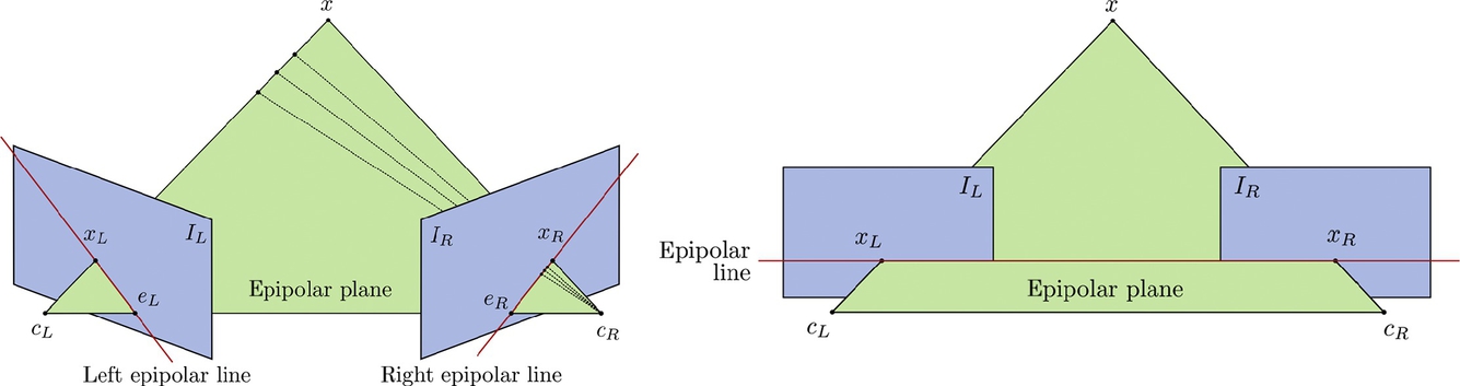
The system proposed by Bätz et al. [75] is comprised of two cameras and two workflows. In the offline calibration workflow, the response curves of both cameras are estimated. This has to be done only once for a given pair of cameras. The main workflow is comprised of several stages. In the first one, stereo rectification is performed, which results in geometrically transformed images such that a given point in the left view resides on the same scanline as in the right view (see Fig. 3). This simplifies determining correspondences between pixel values, which are performed in the second stage. For measuring similarity between pixel values, zero mean normalized cross correlation (ZNCC) is used as it is resistant to exposure variations. The determined disparity maps are then smoothed to avoid abrupt changes between neighboring pixels.
In the third stage, the disparity map is used to warp the source exposure onto the target exposure. To this end, the target exposure is selected as the one with the fewest number of under- and over-exposed pixels. Backward warping is used which, for every pixel in the target exposure, computes a sampling position from the source exposure. As this is likely to produce noninteger sampling coordinates, bilinear interpolation is used to compute the final color value. Finally, the HDR frame is computed by merging the target exposure with the warped one. However, merging is only performed for pixels that are under- or overexposed in the target exposure, which limits the influence of potential errors that may be introduced in the earlier stages.
Similar to Bonnard et al. [73], the system proposed Selmanovic et al. aspires to generate a stereoscopic HDR video [74]. Their system is comprised of two video cameras with one camera being an HDR camera [92] and the other an LDR one. The goal is to generate the missing HDR frame by using the information from the existing HDR and LDR frames. To this end, three methods are proposed. The first one is based on warping the HDR frame toward the LDR frame based on a disparity map, similar to the method of Bätz et al. [75]. The second method involves directly expanding the dynamic range of the LDR frame using a novel inverse tone mapping approach. The third method is a hybrid of the two in which the well-exposed regions of the LDR frame are expanded and the under- and overexposed regions are warped from the HDR frame. The authors conclude that the hybrid approach produces the highest quality results.
4.3 HDR Sensor Solutions
Various algorithms discussed earlier have been necessitated due to the LDR nature of image sensors. Ideally, using an HDR image sensor would solve the problems of the aforementioned algorithms. While not being the primary focus of this chapter, here we will briefly review HDR sensor solutions for the sake of completeness.
There are several ways to design an HDR image sensor. In general, an image sensor can be considered as an array of photodetectors with each photodetector connected to a readout circuit. There may be an optional layer of optical mask in front of the photodetectors as well. An HDR sensor can be produced by either spatially varying the transmittance of the optical mask [76, 93], by modifying the readout circuitry [94], or by using HDR photodetectors [95].
The idea of using a spatially varying filter resembles that of using a Bayer color filter array to produce color images. However, instead of being selective of the wavelength, spatially varying transmittance filters transmit different amounts of light onto each photodetector. A pioneering work in this direction was proposed by Nayar and Mitsunaga [93], who used a regular array of optical filter elements aligned with photodetectors. The final HDR pixel values are obtained by computing the average of the neighboring pixel values with different exposures. However, this approach results in a slight reduction in resolution, especially in regions that contain sharp edges. Schöberl et al. show that the resolution can be improved if one uses a nonregular pattern for the optical mask due to the sparsity characteristics of natural images in the Fourier domain [76]. In a more recent work, it has been shown that high quality HDR images can be obtained from a single coded exposure using convolutional sparse coding [96].
As for modifying the readout circuitry, several alternatives have been proposed. These are (1) measuring time-to-saturation, (2) performing multiple nondestructive readouts during the capture process, (3) readout with asynchronous self-reset, and (4) synchronous self-reset with residue readout. A quantitative evaluation of these four groups of techniques was conducted by Kavusi and Gamal, who conclude that each technique has different advantages and disadvantages [94].
Finally, an HDR image sensor can be obtained by directly extending the dynamic range of the photodetecting elements. As a reference, we refer the reader to Zhou et al. for a design that involves punchthrough enhanced phototransistors [95].
5 Global Video Deghosting
Global deghosting algorithms are typically concerned with aligning input frames as a whole without considering local object motions. As such, they are suitable to be used if the scene is stationary or the movement is small with respect to the capture rate of the camera.
5.1 View Dependent Enhancement of the Dynamic Range of Video [77]
Among the first global approaches to HDR video deghosting problems, Niskanen presented a global alignment method that produces results that are suitable to be used by computer vision algorithms rather than to be viewed by human observers [77]. Deghosting is achieved by aligning SIFT features [97] with RANSAC sampling [98] to compensate for global motion. Therefore, this technique is only applicable when local motion between the frames is negligible.
The video is generated by combining sequential LDR frames with varying exposure times. A CCD camera was used with linear or known camera response. The acquisition process has been augmented by two techniques that control exposure times adaptively. They are based on the information content. The first technique involves maximizing the entropy of observations;
where O1, …, ON are the real scene (S) observations, H(.) is the entropy of observations, and Δt1, …, ΔtN are the exposure times to be selected.
The second technique maximizes the average SNR for all I pixels in the resulting HDR image:
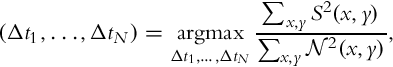
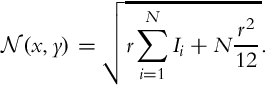
where ![]() with Ii(x, y) being the exposure time normalized and unsaturated signal level for a given pixel in the ith exposure and r is the number of photons required to gain one level of intensity.
with Ii(x, y) being the exposure time normalized and unsaturated signal level for a given pixel in the ith exposure and r is the number of photons required to gain one level of intensity. ![]() , on the other hand, represents the noise level and it is modeled as a sum of the photon shot and quantization noise:
, on the other hand, represents the noise level and it is modeled as a sum of the photon shot and quantization noise:
Using either technique, the optimal exposure times can be computed from frame histograms. It is shown by the author that this technique can select suitable exposure times at 30 FPS among 500 different candidate values.
Once the frames are captured, they are registered using RANSAC sampled SIFT features [97]. This is followed by the construction of HDR frames that are based on modeling light radiation as a Poisson process. In the evaluation of this approach, it was noticed that for small motion, to a certain extent, using the multiple frames without alignment gives better performance than using fewer frames with motion correction.
5.2 Histogram-Based Image Registration for Real-Time HDR Videos [78]
The motivation of this method is to capture and display HDR video in real-time. However, it only considers global translational motion between the frames to be registered. This is done by creating row and column histograms that contain counts of dark and bright pixels in a row or column, and maximizing the correlation between the histograms of two consecutive frames. The two-dimensional search problem is reduced to two one-dimensional searches. The reduction in computation time enables real-time HDR video recording. The robustness of the estimation is increased by Kalman filter application [99].
The image capturing is based on the method of [100]. It achieves efficiency by doing only partial reexposures of a single frame. At first, a full resolution frame is captured at optimal exposure (shutter and gain) setting. This frame is then analyzed to indicate which regions of the frame need reexposures. Usually these regions are frame partials. Additional higher or lower exposures are then captured for these regions only, which reduces the capture and processing times. The reexposures are analyzed and, if needed, additional partial reexposures are captured. The captured images are converted to Y xy color space and all subsequent computations are performed on the Y (luminance) channel.
The process of registration creates a two-dimensional integer translation vector ![]() between a parent exposure and each reexposure. Summing up all translation vectors along the path from an exposure to the base frame, one can calculate an absolute shift between each exposure and the base frame.
between a parent exposure and each reexposure. Summing up all translation vectors along the path from an exposure to the base frame, one can calculate an absolute shift between each exposure and the base frame.
Median threshold bitmaps (MTBs) as described in [10] are used for estimation of translation vectors for a pair of images. As MTBs create an image that contains roughly 50% white and 50% black pixels, it produces similar bitmaps for different exposures. Once the MTBs are computed, the number of black pixels in each column is counted and these counts are collected in column histograms for each MTB.
The MTB algorithm starts with building a regular histogram with 256 bins over the brightness values of Ii−1 and its reexposure Ii. Then the median brightness value mi for reexposure Ii to be used as threshold is determined. Fifty percent of pixels greater than this threshold will be white, while the remaining will be black. The near median pixels are ignored for improved robustness.
The exposure values ei−1 and ei of the images as well as the camera response function f are assumed to be known. To save histogram computation over Ii−1, mi−1 is calculated as follows:
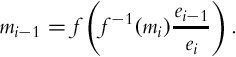
For the purpose of this method, it is sufficient to determine the thresholds mi−1 and mi, and the MTBs are actually not created.
Next, the horizontal and vertical components of the translation vector ![]() between a parent exposure and each reexposure are computed. The horizontal (vertical) component is estimated by computing normalized cross correlation (NCC) between the two column (row) histograms.
between a parent exposure and each reexposure are computed. The horizontal (vertical) component is estimated by computing normalized cross correlation (NCC) between the two column (row) histograms.
Assuming that the width and height of image Ii are wi and hi, respectively, for each column j = 1, …, wi, the column histogram ![]() of exposure Ii is the number of black pixels and is defined as:
of exposure Ii is the number of black pixels and is defined as:
where Ii(j, k) is the pixel value at position (j, k) and |.| denotes set cardinality. Analogously, histogram ![]() counts the number of white pixels. The two histograms are created for Ii−1 in the same fashion. These four histograms are used to estimate the horizontal shift component, xi. This is a search problem that maximizes the NCC between Ii−1 and Ii histograms:
counts the number of white pixels. The two histograms are created for Ii−1 in the same fashion. These four histograms are used to estimate the horizontal shift component, xi. This is a search problem that maximizes the NCC between Ii−1 and Ii histograms:
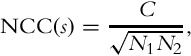
where C, N1, and N2 are computed as follows:

The search range for s can be, for example, ± 64 pixels and for the estimation of xi, the s value that maximizes Eq. (9) is used. Using row histograms, the value of yi is estimated analogously, which results in the final translation vector of ![]() .
.
To incorporate temporal motion estimation Kalman filter is used [99]. To determine the weight of the current translation computation and the preceding trajectory, a novel heuristic is applied. The mean μ and standard deviation σ of the distances d between a pair of consecutive motion vectors (MVs) (![]() ) were precomputed for manually registered images. Assuming Gaussian distribution and near zero mean, over 99% of the MVs are found to be within 3σ from the previous vector. A likely indicator of incorrect measurement is d > 3σ and, in this case, the corresponding shift vector is discarded. On the contrary, if d ≤ 3σ, the state of the Kalman filter is updated using
) were precomputed for manually registered images. Assuming Gaussian distribution and near zero mean, over 99% of the MVs are found to be within 3σ from the previous vector. A likely indicator of incorrect measurement is d > 3σ and, in this case, the corresponding shift vector is discarded. On the contrary, if d ≤ 3σ, the state of the Kalman filter is updated using ![]() as the current state and d as the variance of the measurement. In both cases, the current state of the filter is used as the shift vector.
as the current state and d as the variance of the measurement. In both cases, the current state of the filter is used as the shift vector.
5.3 A Real-Time System for Capturing HDR Videos [79]
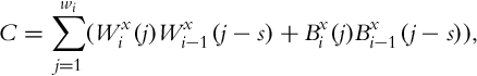
In a more recent work by Guthier et al., a unified real-time system for capturing, registering, stitching, and tone mapping HDR videos is presented [79]. Fig. 4 shows an overview of this HDR video processing system.
The aim of the first step is to only use the exposure times with the highest contribution of information to the generated HDR frame. By minimizing the number of captured images, the processing time is reduced, allowing higher frame rates. This is achieved by defining a contribution function cΔt(E) for each LDR image captured at exposure time Δt. The function computes the contribution of each image captured at Δt to the estimation of radiance E. It is defined as:
where E is the scene radiance, f is the camera response function, and w is a weighting function that measures the well-exposedness of pixel values.
The method computes the optimal exposure time sequence by using radiance histograms, which are generated as a by-product of tone mapping the previous frames. The details of using log-radiance histograms to compute optimal exposure times can be found in [101]. Briefly, the logarithm of the scene radiance histogram contains M bins, (j = 1, …, M), where each index j corresponds to the logarithm of a discrete radiance value: ![]() . Each bin j contains H(j) number of pixels in the HDR image having a log-radiance close to bj. The bins have even spacing in the log domain, thus, Δb = bj+1 − bj. Nonlogarithmic radiance values corresponding to two consecutive bins differ by a constant factor
. Each bin j contains H(j) number of pixels in the HDR image having a log-radiance close to bj. The bins have even spacing in the log domain, thus, Δb = bj+1 − bj. Nonlogarithmic radiance values corresponding to two consecutive bins differ by a constant factor ![]() . The optimal exposure times are selected such that the most frequent radiance values are well-exposed in at least one LDR image. This is obtained by ensuring that the peaks of the contribution functions in each exposure coincide with the histogram peaks as shown in Fig. 5. For a different exposure time Δt′, the corresponding contribution function is computed by simply shifting the original function to another position in the histogram. Therefore, the corresponding exposure times are computed by moving the contribution function over the histogram peaks and deriving the corresponding exposure time by using the following formula:
. The optimal exposure times are selected such that the most frequent radiance values are well-exposed in at least one LDR image. This is obtained by ensuring that the peaks of the contribution functions in each exposure coincide with the histogram peaks as shown in Fig. 5. For a different exposure time Δt′, the corresponding contribution function is computed by simply shifting the original function to another position in the histogram. Therefore, the corresponding exposure times are computed by moving the contribution function over the histogram peaks and deriving the corresponding exposure time by using the following formula:
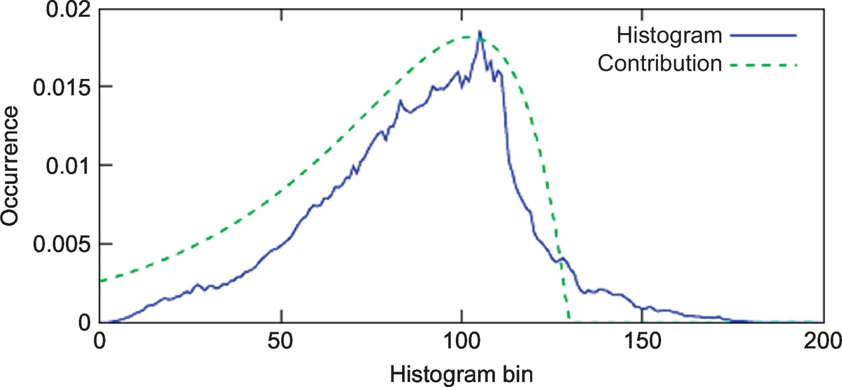
where the contribution vector is shifted by a number of s bins. The computation of new exposure times is repeated until the whole histogram is covered. With this approach, only those LDR images which accurately measure the scene radiance are captured.
The described algorithm for computing exposure times has two problems. The first problem is that the algorithm assumes perfect scene histograms. However, perfect histograms are not available for real-time videos. The problem of imperfect histograms is handled by choosing the first exposure time such that its contribution peak covers the highest radiance bin of the histogram. The reason for choosing the first exposure time in such a way is the fact that underexposed images have more accurate information than overexposed ones. This is because in underexposed images, dark pixels are a noisy estimate of the radiance in the scene, and this noise is unbiased. However, overexposed pixels always have a maximum pixel value, regardless of how bright the scene actually is.
The second problem is flicker that occurs due to the changes in exposure time sequence over time. Furthermore, if the camera is running in a sequence mode (i.e., a sequence of exposure parameters are sent only once and are then repeatedly used throughout the capture), any change in exposure time sequence requires an expensive retransmission of the parameters to the camera. To avoid this, a stability criterion is enforced. This criterion ensures that the new exposure time sequence is only retransmitted when the computed sequence is different from the previous sequence for a number of successive frames. With this approach, temporal stability is also achieved.
The second stage of the proposed system is the alignment of the successive frames, which utilizes the algorithm described in Section 5.2. Once the frames are aligned, HDR stitching is performed using the radiance map recovery technique of Debevec and Malik [4].
The last stage of the system is tone mapping of generated HDR frames. The aim is to apply a tone mapping operator designed for still images while taking measures to avoid flicker. To this end, the average brightness of tone mapped frames is adjusted to be closer to the preceding frames.
6 Local Video Deghosting
Unlike global methods, local deghosting algorithms consider both camera and object motion. Therefore, in general, the algorithms presented in this section are more sophisticated than the former.
6.1 High Dynamic Range Video [80]
This algorithm is considered to be the first approach to generate HDR videos using off-the-shelf cameras by alternating frames between short and long exposures. It is comprised of the following three steps: (1) frame capture using automatic exposure control, (2) HDR stitching across neighboring frames, and (3) temporal tone mapping for display.
6.1.1 Capture
In the capture stage, the exposure settings alternate between two values that are continuously updated to incorporate scene changes. This is done by calculating scene statistics on a subsampled frame. The ratio between the exposures varies from 1 to a maximum specified by the user. It has been observed that the maximum value of 16 generates good results, in terms of both recovering the dynamic range and compensating for the motion.
6.1.2 HDR Stitching
The goal of this stage is to create an HDR frame by using information from the neighboring frames. First, gradient-based optical flow is used to unidirectionally warp the previous/next frames to the current frame. Then the warped frames are merged with the current frame in the well-exposed regions of the latter. The over- and underexposed regions of the current frame are bidirectionally interpolated using optical flow followed by a hierarchical homography algorithm to improve the deghosting process. The details of this workflow are explained as follows.
Unidirectional Warping. In this stage, a flow field is computed between the current frame, L, and its neighboring frames S− and S+. However, to compensate for the exposure differences, the neighboring frames are first “reexposed” using the camera response curve and the exposure value of the current frame. For computing the optical flow, a variant of the Lucas and Kanade technique [102] in a Laplacian pyramid framework [103] is used. After computing the optical flow, the neighboring frames are warped to obtain ![]() and
and ![]() .
.
Bidirectional Warping. This stage is used to estimate the overexposed regions of the current frame (or underexposed if the current frame is a short frame). Because the current frame cannot inform the flow computation in these regions, a bidirectional flow field is computed directly between the previous and the next frames. Using these flow fields, an intermediate frame is computed and this is called as ![]() . This intermediate frame is then reexposed to match its exposure to the current frame. This reexposed frame is called
. This intermediate frame is then reexposed to match its exposure to the current frame. This reexposed frame is called ![]() . Next, an hierarchical homography is computed between the current frame L and
. Next, an hierarchical homography is computed between the current frame L and ![]() . The result of this homography also results in a flow field due to its hierarchical nature. This flow field is added to the original bidirectional flow field to compute the final flow field. S− and S+ are then warped using this flow field to obtain
. The result of this homography also results in a flow field due to its hierarchical nature. This flow field is added to the original bidirectional flow field to compute the final flow field. S− and S+ are then warped using this flow field to obtain ![]() and
and ![]() .
.
Radiance Map Recovery. The next step is to combine the current frame with the four auxiliary frames that were generated. To this end, the following steps are applied, assuming the current frame is a long exposure:
• Using the response function, for all images (L, ![]() ,
, ![]() ,
, ![]() , and
, and ![]() ) compute radiance images (
) compute radiance images (![]() ,
, ![]() ,
, ![]() ,
, ![]() , and
, and ![]() ).
).
• Overexposed pixels in the final radiance map are filled in with bidirectionally interpolated pixels from ![]() to
to ![]() . To avoid possible blurring, pixels from solely the previous frame
. To avoid possible blurring, pixels from solely the previous frame ![]() are used. Only if they happen to be inconsistent with the current frame (too low to saturate in the current frame) then the pixels from
are used. Only if they happen to be inconsistent with the current frame (too low to saturate in the current frame) then the pixels from ![]() are used.
are used.
• The radiance map in other regions is computed as a weighted blend:
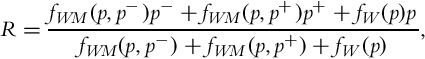
where the pixels p, p−, and p+ come from ![]() ,
, ![]() , and
, and ![]() , respectively. The weighting function fW(.) is based on Mitsunaga and Nayar [104] and fM(.) is used to attenuate large pixel value differences. It is defined as:
, respectively. The weighting function fW(.) is based on Mitsunaga and Nayar [104] and fM(.) is used to attenuate large pixel value differences. It is defined as:
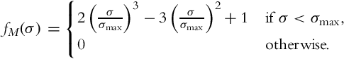
Here, σmax is set to a value that corresponds to 16 gray levels in the longest exposure. Finally, fWM(p, q) = fM(|p − q|)fW(p).
If current exposure is the short one, the same algorithm is used but in the second step underexposed pixels are discarded.
6.1.3 Temporal Tone Mapping
For tone mapping the generated video, Reinhard et al.’s photographic tone mapping operator is used [105]. The computation of log-average luminance is slightly modified to include multiple frames in the spirit of reducing temporal flicker:
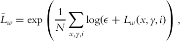
where (x, y) are the spatial indices, i is the frame index, and Lw(x, y, i) denotes the radiance value at pixel (x, y) in frame i. Only the current frame and the previous frame are used during this spatiotemporal averaging. Finally, ϵ is a small value used to avoid singularity for zero radiance pixels.
6.2 Video Matching [82]
Sand and Teller introduced an algorithm for spatiotemporal alignment of a pair of videos [82]. The input of the proposed algorithm is two videos, which may have been recorded with different exposures. Of these two videos, one is marked as the primary (reference) and the other as the secondary. The output is a modified secondary video whose pixels have been brought to temporal and spatial alignment with the primary video. The proposed method is not specialized to HDR video, but it has been shown that it can be used to create HDR videos as well.
6.2.1 Spatial Alignment
Given a primary input frame I1 and a secondary input frame I2, the image alignment algorithm begins by detecting the feature points in both frames using Harris corner detector [106]. The initial matches from I1 for each feature point in I2 are found according to the similarity of nearby pixel values around each feature point.
In the next step, the best matching correspondences are found by maximizing a weighting function, wi, that includes two terms namely pixel matching probability, Pi, and motion consistency probability, Mi:
The pixel matching probability is measured by calculating a pixel matching score across a square region R around the corresponding feature points in two frames. However, instead of comparing the primary frame with the secondary one directly, two auxiliary frames namely, ![]() and
and ![]() , are computed by taking the minimum and maximum of 3 × 3 regions around each pixel. This makes the algorithm more robust against small differences between pixel values:
, are computed by taking the minimum and maximum of 3 × 3 regions around each pixel. This makes the algorithm more robust against small differences between pixel values:

where (u, v) is the offset between the points, which was computed earlier. This dissimilarity score is aggregated over each color channel to determine the final dissimilarity score of each correspondence, di. The final pixel matching probability is computed as:
where ![]() is a zero-mean normal distribution and σpixel is set to 2.
is a zero-mean normal distribution and σpixel is set to 2.
The motion consistency probability term measures the smoothness of the offset vectors. To this end, the authors first estimate a dense motion field, u(x, y) and v(x, y), from the MVs between the correspondences. This dense field is computed by a modification of the locally weighted linear regression algorithm [107] and is called adaptive locally weighted regression. The MV at each pixel is computed by fitting a Gaussian kernel to the nearby feature points. The width of this kernel is inversely proportional to the number of nearby feature points. That is, if a pixel is surrounded by many feature points, the kernel width is reduced. On the other hand, if the feature points around a pixel are sparse, larger kernel widths are employed. The MV is then computed as a weighted average of these kernel functions with the weight of each kernel determined by the correspondence score, wi. Motion consistency is then given by the similarity of these estimated MVs, ![]() , from the previously assigned MVs, (ui, vi):
, from the previously assigned MVs, (ui, vi):
After the initial matches are found, the correspondences between the feature points are improved iteratively by checking the pixel matching score of the pixel at location predicted by ![]() , and several feature points around which are detected by the corner detector. For each candidate correspondence, the proposed algorithm applies a local motion optimization using the KLT method [102, 108]. When the iteration converges to a good set of correspondences, a dense correspondence field is obtained using the adaptive locally weighted regression.
, and several feature points around which are detected by the corner detector. For each candidate correspondence, the proposed algorithm applies a local motion optimization using the KLT method [102, 108]. When the iteration converges to a good set of correspondences, a dense correspondence field is obtained using the adaptive locally weighted regression.
6.2.2 Temporal Alignment
The alignment algorithm discussed earlier is used as the core of a video matching algorithm, which tries to align two videos temporally and spatially. First, each frame in the secondary video is matched to a nearby frame in the primary video. This is accomplished by minimizing the following cost:
where i and j are the frame indices, pi, j is a parallax measure, and mi, j is simply the mean correspondence vector magnitude. λ, which is set to five, is used to control the relative influence of the two terms.
The parallax measure is a measure of depth discontinuity between the frames. Given a pair of correspondences, the difference of the Euclidean distance between them in the first image and the second image is proposed as a suitable measure of these discontinuities. pi, j is computed by averaging this difference for all pairs of correspondences.
Finally, instead of comparing a given frame in the secondary video with all frames in the primary video, an optimized search is employed. This involves computing Di, j for several nearby frames and then fitting a quadratic regression function to the obtained values. The search is then conducted around the frames for which this quadratic function is minimum. Once the matching frame is found, a dense flow field is computed by using the image alignment algorithm described earlier.
6.2.3 HDR Reconstruction
In order to produce an HDR video, this algorithm is applied on a pair of input videos with different exposures after local contrast and brightness normalization [109]. The output pair of aligned videos may be merged using a standard HDR reconstruction method, such as the algorithm of Debevec and Malik [4]. In order to obtain a satisfactory result, the viewpoint must not change significantly between the two input videos. In addition, this algorithm is more successful at recovering the dynamic range of the background rather than the moving objects because the dense correspondence fields are smoothed out to mostly account for the global motion in the input frames.
6.3 HDR Video Through Fusion of Exposure Controlled Frames [110]
Youm et al. [110] proposed a technique that employs a novel exposure control method in addition to ghost removal. The proposed method adaptively selects the exposure times of the individual frames during the acquisition of an LDR video with alternating long and short exposures. After the acquisition, the pyramid-based image fusion method of Burt and Adelson [111] is used for the fusion of the captured frames.
The exposure control method adaptively selects the exposure time of the next frame, using the information available in the current frame, and it is based on the adaptive dynamic range imaging method of Nayar and Branzoi [112]. The algorithm uses two user-set parameters: the saturation level Zsat and the desired intensity level range [Zdes −ΔZ, Zdes + ΔZ]. The exposure time of the current frame, Δti, is determined from the exposure time of the previous frame with the similar exposure, Δti−2, using the following set of rules assuming that the current frame is a short exposure:
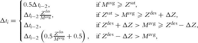
where Mavg is the average intensity in the bright regions of the scene for short-exposure frames. For long exposures, an analogous set of rules is applied.
In the exposure fusion step, the contributions of a pair of long- and short-exposure frames to the output frame depend on the well-exposedness mask Mwe and the ghost mask Mg. Given a pixel value Zi(x, y) from the long exposure and Zi−1(x, y) from the short exposure, the well-exposedness mask is defined as:
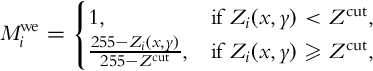
where Zcut is the cut-off intensity for the well-exposedness map. The ghost mask Mg is calculated by comparing the current exposure with the previous corresponding exposure. It takes the value of zero if the absolute pixel intensity difference is larger than 20 for 8-bit input frames and one otherwise.
The output frame is a weighted pyramid-based blending [111] of short and long exposures. The blending weight of the long exposure is ![]() and the blending weight of the short exposure is
and the blending weight of the short exposure is ![]() .
.
6.4 High Dynamic Range Video With Ghost Removal [86]
Recognizing that dense optical-flow based HDR video [80] cannot cope well with occlusions and fast-moving objects, Mangiat and Gibson proposed a novel method that uses block-based motion estimation instead [86]. Their method is comprised of four stages: (1) block-based motion estimation, (2) MV refinement in saturated blocks, (3) HDR reconstruction, and (4) artifact removal. The details of each stage is explained as follows.
6.4.1 Block-Based Motion Estimation
The block-based motion estimation involves two frames, with one being a reference frame and the other the current frame. The goal is to find for each block in the current frame the best matching block in the reference frame. To this end, the current frame is discretized into square blocks of size 16 × 16 and a sliding window of equal size is traversed over the reference frame. The traversal stops when, according a predefined error metric, the difference between the two blocks is smaller than a threshold. Note that this process is commonly used during video compression to exploit the temporal coherence between frames. The difference in the HDR setting is that the consecutive frames are differently exposed, which makes finding correspondences more difficult.
To address the exposure difference, Mangiat and Gibson first reexpose the short exposure to match the long exposure (or vice versa):
where g is the logarithm of the inverse camera response function, i.e., ![]() . Next, two unidirectional motion fields are computed between the current frame (long exposure) and the neighboring frames (previous and next short exposures). To this end, the authors use the H.264 JM Reference Software1 with Enhanced Predictive Zonal Search (EPZS) [113]. This algorithm optimizes finding correspondences by first considering the most likely predictors for the MVs, such as the median MVs of neighboring blocks and MVs of the neighboring blocks in the previous frame. The algorithm stops if these predictors yield an error term that is smaller than an adaptively set threshold. Otherwise, it continues searching using a fixed pattern. The error term is defined as the sum of absolute differences (SAD):
. Next, two unidirectional motion fields are computed between the current frame (long exposure) and the neighboring frames (previous and next short exposures). To this end, the authors use the H.264 JM Reference Software1 with Enhanced Predictive Zonal Search (EPZS) [113]. This algorithm optimizes finding correspondences by first considering the most likely predictors for the MVs, such as the median MVs of neighboring blocks and MVs of the neighboring blocks in the previous frame. The algorithm stops if these predictors yield an error term that is smaller than an adaptively set threshold. Otherwise, it continues searching using a fixed pattern. The error term is defined as the sum of absolute differences (SAD):
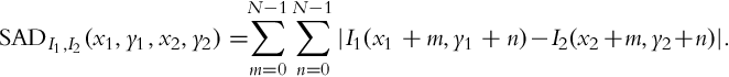
Here, I1 and I2 represent the images, N the square block size, and (x1, y1) and (x2, y2) are the coordinates of the blocks to be compared. Typically, the coordinate pairs that yield the smallest SAD value are assumed to be matching and an offset, (vx, vy), is computed from their difference. This difference is termed as the motion vector. For color images, this search is conducted for both luma and chroma components. Mangiat and Gibson perform this search for both the previous and the next frames of the current frame, and for each block, choose the frame that has the smallest SAD value. To this end, two pieces of information are stored for each block of the current frame: (1) the MV and (2) the label of the previous or the next frame for which this MV is valid. It is also stated by the authors that the estimated MVs can be used to estimate the global camera motion (if any) by using a least squares approach.
EPZS algorithm works well for properly exposed regions. However, for saturated blocks, the current frame does not have sufficient information to guide this unidirectional search. A saturated block is defined as one for which more than 50% of its pixels are above (or below) a threshold. For these blocks, a bidirectional search is performed directly between the previous and the next frames. However, the MVs of the neighboring unsaturated blocks of the current frame inform this search to ensure that the MV of a saturated block is not vastly different from the MVs of neighboring unsaturated blocks. Assuming that the block (x, y) is saturated in the current frame,2 the coordinates of the matching blocks in the previous and the next frame are computed by (x1, y1) = (x, y) + (vx, vy) and (x2, y2) = (x, y) − (vx, vy), respectively. These coordinates can be computed by finding an (vx, vy) value which minimizes:
where Ip and In denote the previous and the next frames, (vmx, vmy) denote the median of the MVs of neighboring unsaturated blocks, and λ is a factor, which determines the relative contribution of the first (data) and the second (smoothness) terms. To compute the median MV, the labels of unsaturated blocks in the 5 × 5 neighborhood of the saturated block are tallied, and the frame (previous or next) with the highest count is selected as the reference. The median MV is then found as the median of the MVs of blocks that are labeled with this reference. Finally, ± represents the operation to be applied depending on whether the reference is selected as the previous or the next frame. Once a saturated block is fixed, it is marked as unsaturated so that it can also inform neighboring saturated blocks. This way larger holes (saturated regions) are gradually filled.
6.4.2 MV Refinement in Saturated Blocks
It is possible that the previous matching algorithm produces incorrect correspondences between blocks. This problem is most pronounced for saturated blocks as for these blocks, the information from the current frame is not used at all. However, although these saturated blocks are not informative, one can still estimate the minimum (or maximum) pixel values that could exist in a matching block. Assuming that the current image is the long exposure and the reference is either the previous or the next short exposure, a saturated pixel of the current exposure should not have been matched with a reference pixel that is too dark to saturate in the current exposure. If this happens, this match is likely to be erroneous.
Therefore, in this stage of the algorithm, the authors determine the minimum pixel value that is valid as:
Any pixel that is smaller than this value in the reference exposure cannot be the correct match for the saturated pixel in the current exposure. Similarly, if the current exposure is a short exposure, a maximum valid value is computed as:
The erroneous pixels are identified to be those that are smaller than ![]() if the current frame is a long exposure and greater than
if the current frame is a long exposure and greater than ![]() if it is a short exposure. Once these pixels are located, their MVs are updated using their eight immediate neighbors and eight nearest neighbors from the adjacent blocks. This amounts to choosing an MV that maximizes the following weight function:
if it is a short exposure. Once these pixels are located, their MVs are updated using their eight immediate neighbors and eight nearest neighbors from the adjacent blocks. This amounts to choosing an MV that maximizes the following weight function:

where Ir represents the reference exposure and qk the 16 candidate pixels from which one of the MVs will be selected. The r(p, qk) term represents the spatial distance and therefore, nearby pixels are favored. The c(p, qk) term, on the other hand, is a color similarity term based on the idea that pixels that are similar in color should have similar MVs. The refinement process is illustrated by an example in Fig. 6.
6.4.3 HDR Reconstruction
This stage of the algorithm merges the current exposure and the estimated exposure using Debevec and Malik’s algorithm [4]:
where w is a triangular weighting function and P is the number of exposures, respectively. The generated HDR image is then tone mapped using Reinhard et al.’s photographic tone mapping operator [105].
6.4.4 Artifact Removal
Given the block-based nature of the algorithm, it is possible that blocking artifacts will appear at the block boundaries. In this stage, the color information of the current frame is used to fix these artifacts. This is achieved by filtering the tone mapped HDR image, using a cross-bilateral filter (CBF) in which the edge information is taken from the current frame [114]. This produces a filtered image with edges smoothed out if they do not exist in the current frame, such as the edges caused at block boundaries. To identify these regions, the filtered image and the original tone mapped HDR image are compared using perceptual color difference and SSIM [115] metrics. If the color difference is greater than a threshold or if the SSIM score is less than a threshold, the tone mapped HDR pixel is replaced by the corresponding pixel in the filtered image. However, if the current frame is saturated for these pixels, the original tone mapped pixel value is not changed.
6.5 Spatially Adaptive Filtering for Registration Artifact Removal in HDR Video [88]
A follow-up work by Mangiat and Gibson proposes to improve the artifact removal stage of their previous algorithm. As discussed in the previous section, the artifact removal stage involved applying a CBF to fix the block artifacts:
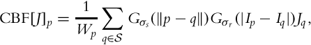
where ![]() is a neighborhood around pixel p. Here, the tone mapped image J is filtered by using the edge information in frame I.
is a neighborhood around pixel p. Here, the tone mapped image J is filtered by using the edge information in frame I. ![]() denotes a Gaussian function with standard deviation σs and likewise for
denotes a Gaussian function with standard deviation σs and likewise for ![]() . Wp represent the sum of all weights. This process blurs across the edges of image J if those edges are not present in image I, e.g., the edges caused by blocking artifacts.
. Wp represent the sum of all weights. This process blurs across the edges of image J if those edges are not present in image I, e.g., the edges caused by blocking artifacts.
Recognizing that artifacts are most likely to occur in large motion regions, the authors propose the modify the standard deviation of the range kernel as:
where α is a user parameter used to adjust the amount of smoothing.
However, this modification cannot fix registration errors that may occur in saturated regions as, in these regions, the current frame does not have any edge information. Therefore, the authors propose a second modification to use the edge information in the tone mapped HDR frame directly for the saturated regions of the current frame. This is formulated as follows:
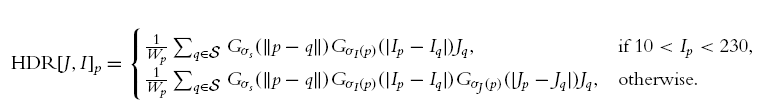
In other words, in regions where the current frame is well-exposed, the tone mapped frame has no influence on the filter. In these regions, the adaptive version of the CBF is used. However, in the saturated regions of the current frame, the tone mapped frame itself is used to smooth out potential registration errors. An additional benefit of this approach is that it obviates the need to perform perceptual color similarity or SSIM computations as the final tone mapped frame becomes the filtered frame itself.
6.6 Filter-Based Deghosting for Exposure Fusion Video [83]
In their work, Chapiro et al. [83] present a method to deal with ghost artifacts based on the exposure fusion approach of Mertens et al. [116]. The proposed method addresses small-scale movements rather than fast object and camera motions. For improving the quality of the input video by eliminating ghost artifacts on object boundaries, a ghosting term is included in addition to the contrast, saturation, and well-exposedness terms of the exposure fusion algorithm. This term reduces the contribution of the motion-affected pixels.
The proposed method begins with applying a multiresolution global registration to each pair of consecutive input frames. In order to detect the pixels that may cause ghost artifacts, low-pass Gaussian filters are applied to the input frames, followed by high-pass Laplacian filters. The ghost term for a specific pixel is calculated by subtracting the SAD from one around a rectangular region in each pair of input frames.
We note that this method does not generate an HDR video, but rather, a better exposed LDR video by directly merging the input frames similar to Youm et al. [110]. Therefore, it does not require information, such as the camera response and exposure times.
6.7 Toward Mobile HDR Video [81]
Castro et al. [81] presented a method of reconstruction of HDR video for hand-held cameras as an extension of a similar earlier work [84]. Because the method is based on histograms, it is of low computational cost and thus, suitable for less powerful processors, such as mobile phones. The proposed algorithm initially captures a multiexposure sequence on Nokia N900. Then the captured exposures are transferred to a desktop computer to generate HDR videos. Finally, the constructed HDR videos are tone mapped to enable visualization on LDR displays. The proposed method of generating HDR video has three steps: (1) photometric calibration, (2) multiresolution alignment, and (3) radiance map estimation.
For photometric calibration, the method takes a sequence of three (or possibly more) exposures Fi as input, where ![]() Exposure
Exposure ![]() is constant for all i and is determined before capture, using the auto-exposure feature of the camera.
is constant for all i and is determined before capture, using the auto-exposure feature of the camera. ![]() and
and ![]() are exposures of twice and half the exposure value of
are exposures of twice and half the exposure value of ![]() , respectively, for all i. Photometric calibration relies on pixel correspondences between pixels from different frames. The authors assume that exposure changes preserve monotonicity of pixel values and define the radiance mapping MP, Q between two consecutive frames, P and Q as:
, respectively, for all i. Photometric calibration relies on pixel correspondences between pixels from different frames. The authors assume that exposure changes preserve monotonicity of pixel values and define the radiance mapping MP, Q between two consecutive frames, P and Q as:
where pi and qi represent the corresponding pixels between two frames. Radiance map is then reconstructed by using the approach described in Mitsunaga and Nayar [104].
However, prior to constructing the radiance map, the exposures must be first brought into global alignment. This global alignment is performed by applying Ward’s MTB registration method [10].
Finally, the removal of ghost artifacts is achieved by analyzing the variance of radiance values over the corresponding pixels of aligned images in Fi. Four radiance maps, ![]() for j = 1, 2, 3, 4 are generated for each Fi. The first three radiance maps are simply the original frames converted to the radiance domain, and the last one is the reconstructed HDR image after global alignment. The first three radiance maps are then updated based on the magnitude of the variance. If the pixel variance is low, the HDR frame is given more weight, whereas for high-variance pixels, the original pixel values are prioritized.
for j = 1, 2, 3, 4 are generated for each Fi. The first three radiance maps are simply the original frames converted to the radiance domain, and the last one is the reconstructed HDR image after global alignment. The first three radiance maps are then updated based on the magnitude of the variance. If the pixel variance is low, the HDR frame is given more weight, whereas for high-variance pixels, the original pixel values are prioritized.
6.8 Patch-Based High Dynamic Range Video [85]
The main contribution of this method, which arguably produces the highest quality deghosting results, is a judicious combination of optical-flow [80] and patch-based [62] HDR image synthesis algorithms. For the capture process, the input is assumed to be N LDR images alternating between M different exposures (Lref, 1, Lref, 2, …, Lref, N). The task is to generate the N HDR frames (Hn, n ∈ 1, …N). For each frame, additional (M − 1) missing frames are synthesized (for all but the reference frame).
Although [62] works very well for still images, it is not suitable for HDR video due to lack of temporal coherency. Also, this algorithm fails if a large region of the image is under- or over-exposed. Thus, the direct application of [62] is not suitable. Therefore, the following modified energy function is proposed:
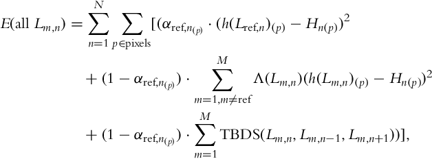
where h(.) converts LDR images to the linear radiance domain, α is an approximation of how well a pixel is exposed, and Hn is an HDR frame. Λ in the second term is weighted triangle function used for merging [4]. The third term, temporal bidirectional similarity (TBDS), adds temporal coherence between the estimated exposures:
with BDS is proposed in [117]:

where patch center in pixel p is marked by s(p) (source) and t(p) (target) and function D is the sum of the squared differences (SSD) between s and t. Here, ![]() approximates the optical flow at pixel p from the source to target and
approximates the optical flow at pixel p from the source to target and ![]() scales the search window. Note that for improved efficiency, the search is conducted around the regions indicated by an initial optical-flow estimation. In summary, the proposed method contains the following three main steps:
scales the search window. Note that for improved efficiency, the search is conducted around the regions indicated by an initial optical-flow estimation. In summary, the proposed method contains the following three main steps:
Initial motion estimation. During this stage, motion is roughly estimated in both directions for consecutive frames (![]() and
and ![]() ). For global motion estimation, a planar similarity model and for local motion, optical-flow is used. The accuracy of this step influences the size of the search window in the next step.
). For global motion estimation, a planar similarity model and for local motion, optical-flow is used. The accuracy of this step influences the size of the search window in the next step.
Search window map computation. A window size of ![]() and
and ![]() is computed for every flow vector. This window is used to refine the initial motion estimate.
is computed for every flow vector. This window is used to refine the initial motion estimate.
HDR video reconstruction. A two-stage iterative method is utilized in which the first stage minimizes the last term in Eq. (34), and the second stage minimizes the first two terms. These two stages are performed in succession until convergence. This produces all of the missing frames and the corresponding HDR image at each time instance.
6.9 A MAP Estimation Framework for HDR Video Synthesis [87]
One of the main difficulties in HDR video synthesis is estimation of accurate MVs between a sequence of multiexposures captured at different shutter speeds. Li et al. [87] proposed a maximum a posteriori (MAP) estimation framework for HDR video synthesis that does not use optical flow calculation for motion estimation. The proposed algorithm is an extension of the rank minimization-based HDR imaging (RM-HDR) [42, 50, 118].
The framework is based on an image acquisition model defined as follows: It is assumed that a pixel value z is defined as z = g(aΔt) + n, where a is the radiance value, Δt is the exposure time, g(⋅) is the response function, and n is a Gaussian random noise. The conditional probability of z given a is defined as:
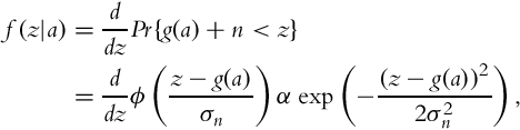
where σn is the standard deviation of n, and ϕ is the cumulative distribution function of the standard Gaussian distribution.
The model generates an aligned background and computes the foreground radiance simultaneously. To solve the problem of scene motion, each exposure is separated into foreground and background regions. Initially, a binary matrix S ∈{0, 1}KxN, where K is the number of pixels in each frame and N is the number of exposures is constructed as:
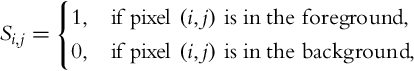
where (i, j) corresponds to the ith pixel in the jth frame.
A probabilistic model for S is then constructed as a Markov random field under the assumption that interactions of a given pixel with all others are entirely described by its neighbors. The probability distribution function that can be considered as the prior probability of S is then defined as:
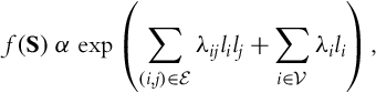
where ![]() and
and ![]() are the set of vertices and edges of the graphical representation of S, respectively, λij and λi are edge interaction costs and vertex weights, and li ∈{−1, 1} is the latent variable corresponding to the ith pixel in S. We refer the reader to Lee et al. [119] for a more detailed description of S and setting the values of parameters λij and λi.
are the set of vertices and edges of the graphical representation of S, respectively, λij and λi are edge interaction costs and vertex weights, and li ∈{−1, 1} is the latent variable corresponding to the ith pixel in S. We refer the reader to Lee et al. [119] for a more detailed description of S and setting the values of parameters λij and λi.
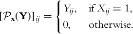
Next, the radiance matrix A for the synthesized HDR video is defined as a combination of the foreground C and background B matrices:
where ![]() is a sampling operator defined as:
is a sampling operator defined as:
Since B, C, and S are unknown, they need to be estimated. Their estimation is defined as a MAP estimation problem:
where D := [vec(I1), vec(I2), …, vec(IN)] corresponds to the scene observation matrix, where each Ik denotes the observed radiance map of the kth frame obtained by using the inverse camera response function as defined in Debevec and Malik [4], and f(S, B, C|D) corresponds to the joint probability of S, B and C, given D. The authors rewrite the estimation problem defined in Eq. (41) as:
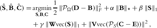
where Ω is the support of the well-exposed background, W is the weighting matrix responsible for interactions between neighboring pixels, and α, β, γ > 0 are constant parameters used to control the relative importance between each term. To solve Eq. (42), an iterative optimization over each variable, S, B, and C, is performed until convergence. More detailed description on the derivation and solution of Eq. (42) can be found in [87].
6.10 Motion Aware Exposure Bracketing for HDR Video [120]
Gryaditskaya et al. [120] introduced a real-time adaptive selection of exposure settings and an off-line algorithm for the reconstruction of HDR video, which is specifically tailored for processing the output of the proposed adaptive exposure approach.
First, the authors present the results of a psychophysical experiment for comparing the relative importance of limited dynamic range vs. ghosting artifacts, because there is a trade-off between the two in multiexposure HDR acquisition. As a result of this experiment, the authors find that the effect of ghosting artifacts is much more significant than that of the limited dynamic range on the perceived quality.
Next, the authors introduce their metering algorithm for the detection of optimal exposure times for minimizing ghosting, while maximizing dynamic range. The first two frames with long and short exposures are captured with the built-in metering system of the camera. The pixel intensities in the frame with shorter exposure are adjusted to the longer exposure. Then, the Hierarchical Diamond Search of Urban et al. [121] is used to estimate the motion between frames.
After calculating the motion field, the dominant MV for a frame is found by using the block-based recursive weighted least-squares method. The blocks which follow the dominant MV are marked as dominant motion regions (DMRs), while other blocks are marked as local motion regions (LMRs).
Placing priority on deghosting while extending the dynamic range, a requirement found from the psychophysical experiment, is satisfied by fulfilling the following two conditions while adaptively selecting the best estimate ![]() for the exposure time of the next frame Δti+1:
for the exposure time of the next frame Δti+1:
1. A specific pixel must be properly exposed in at least one of the subsequent exposures.
2. At least a certain percentage of pixels must be properly exposed in both of the subsequent frames.
When these conditions are met, the output HDR is expected to have a dynamic range as high as possible without causing severe ghosting artifacts. Because in order to recover a poorly exposed region from other exposures, at least one of them must be well-exposed (condition 1) and in order to find a reliable correspondence to prevent ghosting between different exposures, at least some of the pixels must be well-exposed in multiple frames (condition 2) because image registration algorithms mostly fail in poorly exposed regions.
The first condition is satisfied by establishing an upper limit on Δti+1:
where [Zlow, Zhigh] is the user-defined pixel intensity range for well-exposedness, such that the pixels whose intensities are lower than Zlow are obtained from longer exposures, and the pixels whose intensities are higher than Zhigh are obtained from shorter exposures.
The second condition is satisfied by applying refinements to ![]() for achieving a desired upper limit on the percentage of overexposed pixels in LMRs and DMRs. The expected number of overexposed pixels in the next frame corresponds to the number of pixels in the current frame whose intensities are larger than
for achieving a desired upper limit on the percentage of overexposed pixels in LMRs and DMRs. The expected number of overexposed pixels in the next frame corresponds to the number of pixels in the current frame whose intensities are larger than ![]() :
:
The percentage of overexposed pixels in LMRs and DMRs is calculated by counting the number of pixels in the current frame whose intensities are larger than ![]() . This operation is performed for different exposure settings provided by the camera. The exposure setting which satisfies the upper limit on Δti+1 and the predefined limit on the percentage of the overexposed pixels in DMRs and LMRs is selected as the value of Δti+1. This process is used for searching for a longer exposure time and searching for a shorter exposure time is an analogous operation.
. This operation is performed for different exposure settings provided by the camera. The exposure setting which satisfies the upper limit on Δti+1 and the predefined limit on the percentage of the overexposed pixels in DMRs and LMRs is selected as the value of Δti+1. This process is used for searching for a longer exposure time and searching for a shorter exposure time is an analogous operation.
Once the whole sequence of frames is captured using the real-time adaptive exposure selection method described earlier, it is processed to produce an HDR video. Because the exposure settings of the captured frames are not periodic and the exposure times are not regularly spaced, available HDR reconstruction algorithms cannot be used without modifications. For this purpose, the authors use the method of Kalantari et al. [85] (Section 6.8) after making necessary modifications to their algorithm.
The method of Kalantari et al. [85] is extended by synthesizing a set of exposures for each frame in the sequence. The exposures in the set are found by recursively searching for the frames with shorter and longer exposure times, which have sufficient spatial overlap with the current frame. Once the exposure stack of each frame is formed, they are merged into HDR frames. The method of Debevec and Malik [4] is modified by introducing a probability of correct match term for the patch-based search of Kalantari et al. [85]. The results of the proposed algorithm are found to be better than the original method of Kalantari et al. [85], when compared using the mean structural similarity index (SSIM) [115] score.