Chapter 3: Preparing Your Data for Multidimensional Models

Multidimensional models are the original OLAP structures supported in SQL Server Analysis Services (SSAS). Starting out as OLAP services over 20 years ago, the tooling is now considered mature by Microsoft and is not planned for any major updates in the foreseeable future. Throughout the years, Microsoft has made significant improvements to Analysis Services and its support for multidimensional models. This includes changes to support dimensional models or star schemas. Today's version of Analysis Services continues to lean heavily on that data modeling pattern.

This chapter focuses on preparing your data. To properly build a multidimensional model, your data should be shaped using dimensional modeling techniques. You will be introduced to dimensional modeling theory, design practices to support those models, and other techniques to support using cubes with SQL Server. Without this data preparation, you will struggle to build cubes that are efficient and performant.

In this chapter, we're going to cover the following main topics:

• A short primer on dimensional modeling
• Designing and building dimensions and facts
• Loading data into your star schema
• Using database views and data source views
• Prepping our database for the multidimensional model
• Let's get started!

Technical requirements

In this chapter, we will be using the WideWorldImportersDW database from Chapter 1, Analysis Services in SQL Server 2019. You should connect to the database with SQL Server Management Studio (SSMS). We will be creating views at the end of this chapter in preparation for building multidimensional models in Chapter 4, Building a Multidimensional Cube in SSAS 2019.

A short primer on dimensional modeling

The foundational architecture for successfully building multidimensional models in SQL Server is the dimensional model or star schema. As Microsoft continued to improve Analysis Services, one of the key elements was embracing dimensional model design as a key element to building cubes. The marriage between dimensional modeling and Analysis Services eventually resulted in a book by the Kimball Group, which combined their concepts with the Analysis Services implementation – The Microsoft Data Warehouse Toolkit. In this section, we will introduce you to the basics of dimensional model design.

Understanding the origin of dimensional modeling

Ralph Kimball is considered the father of the dimensional model. He founded the Kimball Group in the 1980s and coauthored all the books in the Toolkit series. The Kimball Group authored multiple books, conducted thousands of training sessions, and supported the growth of dimensional modeling until it closed its doors in 2015. You can find out more about the Kimball Group on their website at https://www.kimballgroup.com.

Dimensional modeling exists today in response to the need to simplify reporting for end users and report writers. By the time dimensional modeling was introduced, relational database theory was mature and relational database management systems (RDBMS) were optimized to support those normalized data models. The key design principles for normalization are as follows:

• Eliminate duplicate data.
• Make sure all the data in the table is related.

Highly normalized structures involve multiple tables with relationships between them. These databases could be normalized based on normal forms. The most common designs today for transactional systems are in the third normal form.

Let's look at the first, second, and third normal form rules:

• Remove duplicate columns or fields from the table (First normal form rule).
• Create separate tables for related columns and assign a unique primary key (First normal form rule).
• Remove common data elements from a table that apply to multiple rows (Second normal form rule).
• Create relationships between these tables using foreign keys (Second normal form rule).
• Remove all columns not directly related to the primary key (Third normal form rule).

While normalization supports high-performing transactional business needs, it adds a significant amount of complexity when you're trying to build a report on the information. In some cases, dozens of tables may be required to build out a meaningful report in mature, normalized solutions. Furthermore, the database engines built by vendors such as Oracle and Microsoft were designed to optimize this type of interaction with the data.

The complexity of normalization is the impetus for dimensional models and the denormalization of data. This is not a simple design choice. In order to effectively improve the ability and performance of RDBMS solutions so that they return large amounts of aggregated data, specific design considerations were made to support the systems where the data was located, as well as the needs of the business.

For this new model to be successful, it needed to lean on the capabilities – and account for the weaknesses – of the platforms it would be deployed on. The star schema design, with its dimensions and facts, did just that. Indexes and caching capabilities were considered in the design, as well as the simple use of data. While there are hundreds of nuances and variations in the design principles, the core result was an elegantly simple design that could be supported by the systems available when it was created.

Now, we will look at a number of key concepts around dimensional modeling that impact our multidimensional design. Understanding these concepts is important when it comes to prepping your data for a successful multidimensional model or cube.

Defining dimensional modeling terms

Dimensional modeling has its own vernacular. Some of the language carries forward into the cubes themselves. Here are some core terms you should know:

• Dimension: Something you can slice a metric by. The key word here is by; for example, I want to know the sales by country, by month, by salesperson. That statement would result in three likely dimensions – geography, date, and employee.
• Fact: A fact is measurable. It may be able to be summed, averaged, or otherwise aggregated. It is the target of the dimension. A sales fact table could likely have revenue, quantity, and taxes as measures or facts.
• Star Schema: This is the design of the dimensional model. It looks like a star since it has fact tables at the center and the arms of the star as the dimensions. The following is an example of a star schema:

Figure 3.1 – Star schema example from Wide World Importers Data Warehouse

• Grain: The grain of a fact table is effectively the lowest level you can drill to in the data. This is usually defined by combining the dimensions in the table. For example, if the fact table has a daily grain by salesperson, it would aggregate the sales for the salesperson to the day. This would likely add another fact to the table with the count of sales for the day.
• Surrogate Key: These keys are used with the dimensions. Because most data warehouse solutions combine data from multiple source systems, they often have separate keys for the same dimensional item. For example, a CRM solution may have a product ID, which is different from the inventory system. In dimensional models, we strive to have only one product dimension to help related data from various facts in a single solution. Surrogate keys allow us to create a generic key that will be used to represent the same item from multiple systems. This is key to making conformed dimensions, which will be covered in the next section.

Many more terms exist in the world of dimensional modeling, and there are books and other resources that dig into the details. We'll cover a couple more key concepts around dimensional modeling next.

Key dimensional modeling concepts

Dimensional modeling includes some key concepts that have set it apart from traditional relational database modeling techniques through the years. Those concepts must be considered when you're designing your multidimensional model.

Conformed dimensions

Conformed dimensions are one of the key simplifying concepts in the dimensional model design process. Data warehouse solutions often pull data from various source systems. These systems usually handle specific business needs. Continuing with the sales example we used previously, products could exist in the customer relationship management, inventory, and point of sale systems. This would result in three keys and different attributes related to a product in each solution. As the star schema is built out, having one product dimension to support all data will be the key to success within the model. In the following example, I will walk through these three sources and how we could create the conformed dimension.

Product source definitions

The following definitions show the three sources and their product attributes, as well as an example of our Wonderful Widget product:

• Customer Relationship Management (CRM) Product:

  a) Product ID: WW123

  b) Product Name: Wonderful Widget

  c) Product Description: Wonderful Widget that everyone loves

  d) Product Color: <<empty>>

• Inventory Product:

  a) Product ID: 4321

  b) Product Name: Wonderful Widget

  c) Product Source: Joe's Amazing Emporium

  d) Product Storage Requirement: ¼ pallet

• Point of Sale (POS) Product:

  a) Product ID: 8712.12

  b) Product Name: Wonderful Widget

  c) Product Price: $12.00

  d) Product Cost: $8.44

  e) Product SKU: WW1223-001-009

Conforming a product

As you can see, we have different IDs and names. Part of conforming a dimension is understanding what the business wants to see on your reports, as well as making sure that the product dimension has the right information from the sources. Here is one way we could choose to make the product dimension conform with the source we chose:

• Product SID: 79, Surrogate key, not related to any source
• Product SKU: WW1223-001-009, from POS
• Product Name: Wonderful Widget, from Inventory
• Product Description: Wonderful Widget that everyone loves, from CRM
• Product Cost: $8.44, from POS
• Product Price: $12.00, from POS
• Product Source: Joe's Amazing Emporium, from Inventory

Not all the fields we specified previously were required for our data warehouse. One of the keys to good design in this case is related to the cost of storage and performance. When the dimension is loaded, a staging area will likely support the lookups in order to match the keys and updates. By conforming the dimension, we can collect facts into fact tables that can share this dimension, thus making report design simpler and standardized.

Slowly changing dimensions

As you likely noticed, product cost and price attributes likely change over time and can affect calculations throughout the life of a data warehouse. The concept of slowly changing dimensions (SCD) covers this design issue. There are many types of slowly changing dimensions. The most common implementations that can be supported in a cube are as follows:

• SCD Type 0: In this case, we never change the dimension attribute, even if a change comes from the source.
• SCD Type 1: We replace the dimension attribute with the latest value from the source. We retain no history of its previous value. In our product example, the name and SKU are great candidates for this. Typically, we only care about the current name and SKU for our business.
• SCD Type 2: We add a row with the updated attribute and retain its history. This is the most complicated to effectively implement here (there are more complicated SCD types, but they are not in the scope of this book). In order to support the SCD Type 2 attribute, you need to add fields to your dimension table. This typically includes Date Valid From, Date Valid To, Current, and in some cases Deleted. This combination of attributes supports using the correct value at the time the data was valid.

  SCD Type 2

  In my experience, many businesses want the ability to do this, but also do not want it to affect their reporting. I have commonly created a current version of a dimension to support consistent reporting. The SCD Type 2 dimension was used when historical support was required. It is typically more complicated to build reports using Type 2 because a user often sees the changes as bad data if they are not aware of whether the historical support is in place. Use SCD Type 2 only when needed to support a specific business case.

The enterprise data warehouse bus matrix

In the late 1990s, Ralph Kimball introduced the Enterprise Data Warehouse Bus Matrix, or simply the Bus Matrix. It is a simple and elegant way to describe the relationship between dimensions and facts within a dimensionally modeled data warehouse. There are multiple articles on its implementation if you are interested in reading up on them. Here is an example of a bus matrix that is reflective of our current example solution; that is, Wide World Importers:

Figure 3.2 – Bus matrix for Wide World Importers

The bus matrix is implemented in Analysis Services. By designing your underlying database in a dimensional model, you will find it easy to translate that design into your multidimensional model.

Common issues in relational dimensional models

With all the effort that's put into dimensional models, why do we need tools such as Analysis Services? Great question!

RDBMS systems were not specifically designed to support OLAP workloads. The star schema was designed to take advantage of the strengths within an RDBMS, while at the same time simplifying the model for the business. However, relational systems designs were still focused on meeting transactional demands, not reporting demands. Small high-speed transactions are the focus, not large volumes of data, which are aggregated as required for reporting.

SQL Server columnstore indexes

Microsoft released its new columnstore index functionality in SQL Server 2012. This technology has been improved significantly as SQL Server has matured today. Columnstore indexes use the same technology as SSAS tabular models to increase the performance of reporting by storing data in a column-wise pattern. While most normalized systems reduce duplication in tables with related tables, columnstore indexing reduces how many duplicated values can be stored in columns, thus improving performance and improving how the data is compressed. It is ideally suited to support denormalized schemas, such as the star schema.

While improvements have been made to the RDBMS products through the years, SSAS was designed from the ground up to support aggregations and reporting. Multidimensional models support large amounts of data that's highly compressed and optimized for returning aggregated results.

Another reason that SSAS was introduced was to eliminate the use of SQL in writing reports. Integration with Excel made SSAS a favorite tool for business analysts all over the world. They are able to connect to the cube and then use drag and drop features with pivot tables and pivot charts to do a quick analysis of the data, without writing SQL or requesting data from the IT team. This simplified data analysis considerably.

Planning dimensions and facts

Now that the basics around dimensional modeling concepts have been covered, the next step is planning the dimensions and facts for your data warehouse. The following principles need to be kept in mind:

• Know what problem you are trying to solve. You need to know what the business is trying to understand. Your design should understand the various business areas that need to be analyzed.
• Understand the grain. As we noted previously, it is important to know what the grain of each of the fact tables will be. Do you need to support multiple grains? For example, let's say a sale has a total and a date when it occurred. However, if the sale or invoice consists of multiple items, you may need to track your sales at the purchase level (one fact table) and your line items in the sale in a different fact table.
• Build out your bus matrix. You need to understand your facts and dimensions. This will continually change throughout your implementation but understanding your first fact and its dimensionality will help you add facts and know when you need to add dimensions. We often know a few dimensions we need right away, such as customers, products, dates, or locations. Plan your core conformed dimensions out so that you can start the build quickly and expand the capability of your solution with your business needs.

At this point, I will lay out a word of caution: too much time spent in the design process will be counterproductive. Businesses are typically very impatient. If you try to solve everything at the beginning, you will never build anything. Always try to identify how you can make the wins you need iteratively. You should always be delivering more to the business so that they can see your progress and support your efforts as you build out the solution.

Designing and building dimensions and facts

Because our focus is on building a multidimensional model in SSAS, the next few sections will be relatively short, but focused on what you need in order to build out a good star schema using SQL Server 2019.

Column names – business-friendly or designer-friendly?

Without trying to start a war about whether you should have spaces in your column names, I want to call out that this is merely an option. In SQL Server, you can use truly business-friendly names in your tables and columns. Most, if not all, DBAs will argue that this is not a best practice. In order to properly do this, the database object names must be enclosed in brackets. While the name might appear in a nice format on the resulting report, the SQL syntax becomes more complex.

The reserved word conundrum

In every RDBMS system, reserved words exist. This commonly includes words such as NAME, EXTERNAL, GROUP, BULK, and USER. SQL Server has well over 100 of these words. This means that something such as a product name needs to have a fully descriptive name, not just NAME. While you can potentially use reserved words in your table designs, this is not a best practice and should be avoided.

Let's design the product dimension from the work we did previously. We will create the table using both types of syntax and then show you what the query would look like.

Here is the script for the table with spaces in the names:

CREATE TABLE [Dimension].[Product] (

[Product SID] INT NOT NULL

,[Product SKU] NVARCHAR(15) NOT NULL

,[Product Name] NVARCHAR(100) NOT NULL

,[Product Description] NVARCHAR(500) NULL

,[Product Cost] DECIMAL(18,2) NOT NULL

,[Product Price] DECIMAL(18,2) NOT NULL

,[Product Source] NVARCHAR(200) NULL)

Here is the script for the table without spaces in the names:

CREATE TABLE [Dimension].[Product] (

[ProductSID] INT NOT NULL

,[ProductSKU] NVARCHAR(15) NOT NULL

,[ProductName] NVARCHAR(100) NOT NULL

,[ProductDescription] NVARCHAR(500) NULL

,[ProductCost] DECIMAL(18,2) NOT NULL

,[ProductPrice] DECIMAL(18,2) NOT NULL

,[ProductSource] NVARCHAR(200) NULL)

While some data professionals like using underscores in their designs, I typically only use that syntax style to clarify a use or something similar. For example, I use them to clarify that a field has a special use. The surrogate key for the product dimension could be ProductKey or Product_Key. However, I would not use underscores to replace spaces – Product_Short_Name versus ProductShortName. The point of this is that you should settle on a naming convention for your solution and that it should be understandable and simple. The focus should be for others, not you. A data warehouse designed for you may make it easy for you to maintain, but not something the business wants to use.

Now, let's look at those queries against the tables we created previously. The first query does not require brackets for the object names:

SELECT ProductSID, ProductSKU, ProductName

FROM Dimension.Product

The second query does due to the spaces in the names:

SELECT [Product SID], [Product SKU], [Product Name]

FROM Dimension.Product

If you are going to have report writers and business users interacting with your data, I recommend that you don't use spaces. It will be easier to train report writers to handle SQL correctly than to deal with the multitude of issues that will likely be generated using brackets.

One other thing about naming conventions that you should take into consideration is that some developers and database designers using dim and fact as prefixes for the tables. Others use schemas to accomplish the same result. Once again, this is a preference, not a rule. Pick the pattern you want to implement and stick with it. Our example database, WideWorldImportersDW, uses schemas – Dimension and Fact – to clarify the tables.

Dimension tables

Dimension tables should be planned to support the conformed dimension logical design you have. Continuing with the product theme, the product dimension table should have the following fields:

• Product_SID: Surrogate key, identity column, clustered index
• ProductSKU
• ProductName
• ProductDescription
• ProductCost
• ProductPrice
• ProductSource
• Product_ValidFrom
• Product_ValidTo
• Product_Current
• Product_Deleted

This design supports SCD Type 2 functionality. Following the design we have in place, this dimension supports SCD Type 2 for cost, price, and source. The rest of the attributes support the SCD Type 1 design, which overwrites on update. The primary key is the surrogate key in our design. Traditionally, SQL Server developers use identity columns (auto-incrementing integers) for the surrogate key. In SQL Server 2019, the recommendation is to use sequences to auto-populate the key. To wrap up the design, we will add a clustered index to the primary key and cover indexes that support our expected query patterns.

A little bit of information about indexes

Indexes are used to optimize searches and queries in databases. In this section, we mentioned two common types of indexes used in relational databases that support data warehouses. The first is the clustered index. A clustered index is used to order the data in a table. The second is the covering index. A covering index is used to organize data so that you can specifically support queries against a table. Overall, indexes are used to improve the performance of queries in databases.

The rest of the dimensions for any data warehouse you are working on should follow the same basic principles laid out here.

Fact tables

Fact tables typically have metrics and dimension keys. Be aware that this is a fairly simple design. In many cases, fact tables will have additional, non-measurable fields. Our example is a simple design to highlight design patterns. The fact table in our case includes a key for the table, which is effectively a row number. Foreign key constraints are added to each of the dimension keys used in the fact table.

With SQL Server 2019, additional techniques can be used to further improve the design and implementation of the fact table. For example, in our example data warehouse, a similar table, Fact.Sale, was built with a clustered columnstore index instead of a standard clustered index, but only on the primary key fields. The primary key for this table has a unique index applied as well. The rest of the fact tables will use similar design patterns.

Indexing strategies

While indexing strategies are not a primary concern when working with multidimensional models, they have to be considered when completing the star schema. The key impact this has on Analysis Services is data refresh. As data volumes grow, indexes will be required to optimize processing performance for the cube. When designing the star schema initially in SQL Server 2019, the following indexes should be applied to support the expected workload.

Organizing the tables with clustered columnstore indexes will improve the overall performance of processing. This is primarily because a denormalized database design such as a star schema lends itself to many duplicated values in the columns of the tables. This duplication is optimized through compression and memory support and results in better performing queries on larger tables in particular. A key consideration is that the compression and related performance for clustered columnstore indexes is realized on partitions larger than one million rows. If your table has less than one million rows, performance may not be helped as much.

If clustered columnstore indexes are not a good fit for your table, start by creating a standard clustered index on the table. Using the key is the best way to keep the load to the table efficient, but if the data is bulk loaded using a date value or similar pattern, consider expanding the clustered index so that it includes that value. Clustered indexes represent the physical storage order of the table. As such, if the key value is constantly loaded out of order, the table will become fragmented. For dimension tables, using the unique, typically sequential, key for the clustered index makes the most sense.

Traditionally, non-clustered indexes have been at the heart of performance improvements in data warehouse solutions. When designing the star schema, non-clustered indexes are initially used with the foreign keys in fact tables. (Foreign keys are used to match data between tables.) As query performance is evaluated and common patterns for queries are identified, covering indexes are added to tables. Covering indexes have multiple columns in the index. Some columns are ordered, while others are included. This improves read performance in the data warehouse and helps with loading the cube when the indexes are set up to support processing Analysis Services databases.

Plenty of indexing techniques and patterns have been used through the years to support relational databases that have star schemas. Analysis Services uses these optimized databases to process the data in the model. However, these same databases may also be used for reporting or other data analytics purposes. When applying indexes to databases, always consider competing workloads.

Foreign key

Because the work is being done on a relational database platform, enforcing relationships is considered a best practice. Most data warehouses will include this in the design. However, if you experience performance issues during the loading process, you may find significant gains when removing the constraints. I would only recommend this if you need to improve load performance and you can validate that constraint checking is part of the issue. The constraints should be kept if your load process may have orphan records due to load inconsistencies.

These are just a few design considerations you should think about when building your solution so that it supports a multidimensional model. Next, I will walk through some of the loading options you can consider.

Loading data into your star schema

Now that you have your star schema designed, what's next? You need to build a plan so that you can load data from the source systems and get them properly in place in your star schema. In this section, I will give you some pointers to get you going. This is not an exhaustive or complete loading strategy but should help you understand the basics you need to plan.

Staging your data

I recommend that you plan to stage your data in a database prior to loading it into your star schema. The process of lookups and standardization can add significant load on the system that you are loading from. By having a staging database or a staging schema, you can load data from various source systems with minimal transformation. Then, using the resources dedicated to the process, the data can be loaded from staging to the star schema without there being any negative impacts on the source. How often you stage data can be managed based on the needs of the source system.

SQL Server data loading methods and tools

SQL Server has a number of methods and tools you can use to load data into a star schema. I will reference the two most common methods – ETL and ELT – and the most common tools – SQL Server 2019 Integration Services (SSIS) and SQL – used to load star schemas.

When working with any type of data warehouse solution, ETL and ELT are the most commonly referenced patterns. Let's take a look at what each of the letters in ETL and ELT stand for:

• E: Extraction, the process of pulling data from a source system
• T: Transformation, the process of manipulating and shaping data for use
• L: Load, the process of loading data into a destination system

The order of the letters – ETL and ELT – describe when and where the data will be transformed or shaped. ETL is the most traditional solution. This typically involves a specialized tool such as SSIS to be used between the two datasets.

In an ETL solution, to load the star schema from staging, SSIS will connect to the staging dataset, bring the data into the tool, use steps in the tool to manipulate the data, and then load the manipulated data into the star schema. The following is an example of an SSIS package that loads a dimension into the star schema:

Figure 3.3 – Sample data flow task in an SSIS package

The key here is that the most significant transformation work is conducted while the data is in the process of being loaded into the star schema. SSIS and similar tools flow data through and use memory and temporary storage to make changes required to the data along the way.

ELT moves the transformation workload to the destination. This technique has come into fashion more recently as developers seek to use the processing power and capabilities of the destination system to transform data. In this pattern, data is moved from the source to the destination first using the data movement tool of choice (for example, SSIS). Once it has been moved, jobs are initiated that typically use SQL and stored procedures to transform the data into the star schema. If you have your staging database on the same instance or if you're using a schema for staging, this is a popular choice. This allows development teams to focus on fewer coding languages, which helps with ongoing maintenance and staffing.

There is not a right or perfect design choice. More mature solutions have a combination of these techniques, with the goal of being the best option for the job at hand. Whichever path you choose, this section should have given you a basic understanding of the primary options you can use to move and shape your data into the star schema, which is used to support multidimensional models.

Using database views and data source views

So far, the focus has been on prepping the star schema in the relational database so that you can build out the multidimensional model. This section will focus on a design decision that impacts database design, but also impacts how you work with Analysis Services itself. As part of building out a multidimensional model, data source views are created in Analysis Services to serve as the mapping between the relational and multidimensional models:

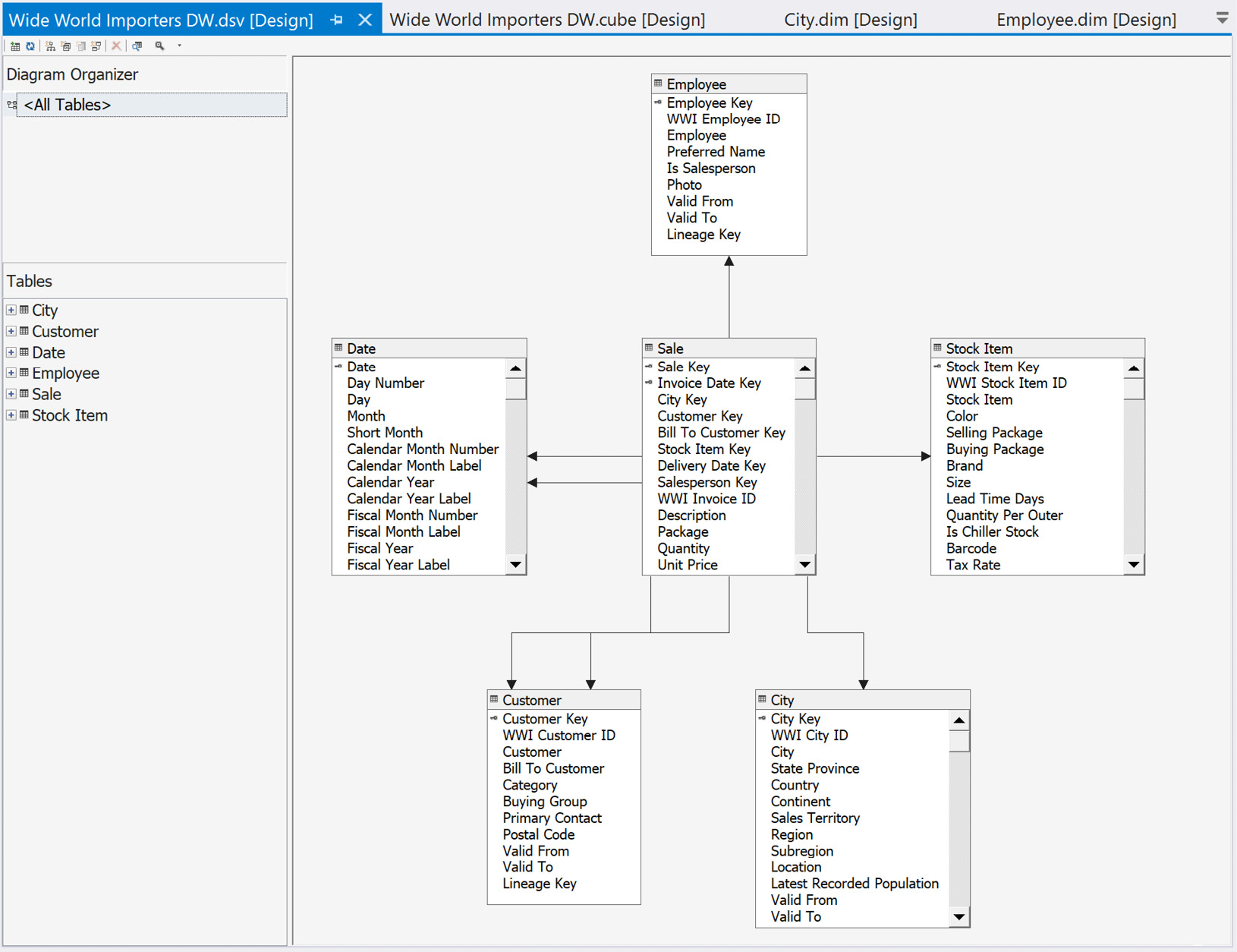
Figure 3.4 – Data source view in SQL Server 2019 Analysis Services from Visual Studio

We will now look at the pros and cons of data source views.

Data source views – pros and cons

Data source views (DSVs) are an integral part of a multidimensional model project. This is where the source data is modeled for the multidimensional model. In the preceding screenshot, the star schema can be clearly seen. The preceding model has been pulled directly from the underlying SQL Server database with no modifications. The key to the preceding statement is no modifications. In my opinion, this is the best way to implement the data source view. However, it is not the only way.

DSVs support the creation of custom tables, fields, and relationships. The end goal is star schema shaped data that can be easily used by the multidimensional model.

Why would you modify the shape of the data here? Some designers make changes here because it is convenient. Changes are made here for the purpose of cube design and do not require any other intervention. Convenience is not a good reason to make changes here. Often, those changes are not well-documented or easy to discover. When the source changes, care must be taken to ensure the DSV also handles these changes. If not, cubes will not process, which creates frustration with the end users or consumers of the cube when it is not available.

The best reason to shape the data in the data source view is when developers cannot easily change or modify database views, as this helps support the star schema model in the underlying database. If this is the reason, then I recommend that you make it the pattern for ongoing work. You will not be able to take advantage of better view design techniques from the database, but it will allow you to make the changes needed to support multidimensional model design. Be aware that complex data source views can significantly impact model processing (loading the data). I recommend only using DSVs when this is the case. The preferred option is to push the view design to the relational database, where management and performance are better.

Database views as an interface layer

The preferred practice is to use database views as an interface layer. There are two principles to take into account – flexibility and protection.

Database views allow you to be flexible in your design. Views can be used to support calculations, aggregations, and column design. In a view, a calculation can be added that will reduce the calculation workload in the cube. For example, the following measures are part of the sales fact: Total Sale, Total Sale with Tax, and Total Sale with Shipping and Tax. They use Total Sale, Total Tax, and Total Shipping as base metrics. These can definitely be calculated in the cube using multidimensional expressions (MDX). However, they will not be pre-aggregated and will degrade performance. If these are precalculated in the view, they will not need calculations to be created in the cube.

This example already works to support aggregation optimization in the cube. Another example is that SUM typically performs better than COUNT in a cube. If each row counts as 1, then adding a column with the value of 1 to the view allows the cube to optimize the aggregation using a sum rather than counting the rows.

Finally, by using a view to cover all tables used in the multidimensional DSV, changes can be made to optimize the underlying tables while guaranteeing there's an interface for the relational model that does not change. This protects the cube from unintentional breakage when you're changing the underlying schema to optimize the database or to change functionality. For example, if a source system changes the way a date is formatted, the view can modify the format so that it matches what is expected in the cube, thereby preventing processing issues. This method also prevents issues caused by core changes in the underlying database, such as fields being added or removed and object name changes (tables or columns).

I recommend using views as the interface or abstraction layer as it will protect the cube from disruption and lead to better user satisfaction. Optimization and aggregation support are helpful as well, but protection is more important.

Prepping our database for the multidimensional model

Everything in this chapter is about prepping the underlying data and database in order to support a multidimensional model. This section presents a hands-on implementation of the views to support the multidimensional model we are going to create.

Wide World Importers Sales

The focus of this book is on Wide World Importers Sales. In particular, the Fact.Sales table will be used as the heart of the schema. The following dimensions are part of our model design:

• City: Dimension.City
• Customer: Dimension.Customer
• Bill To Customer: Dimension.Customer
• Invoice Date: Dimension.Date
• Delivery Date: Dimension.Date
• Item: Dimension.Stock Item
• Salesperson: Dimension.Employee

A total of six tables will be used in the multidimensional model. These tables already exist in our data warehouse, so the next step is to create views that will support the multidimensional model build in the following chapters.

Role playing dimensions

While only five dimension tables support the sales of the star schema, seven dimensions are in the design. Date and customer tables are used twice each in this design. Dimension tables used more than once in a schema are referred to as role playing dimensions. These dimensions use the same data but represent different business relationships in the data. Date is one of the most common role-playing dimensions. In the Wide World Importers Sales fact, both an invoice date and delivery date are used. The underlying shape and content of the date table for both dimensions are identical, but the business purpose or role of the relationship is different. This technique allows data warehouse teams to manage the data while making it available for many purposes.

The data warehouse designers choose a few techniques we have described:

• Using business-friendly names for database objects.
• Using common naming with spaces included in table names and field names.
• Using square brackets [] when referring to objects in the schema. As a best practice, square brackets will be used in all the code to keep the pattern uniform, whether they are needed or not.
• Using database schemas to differentiate fact tables, dimension tables, and staging tables. The [Fact], [Dimension], and [Integration] schemas are already in place and used in the data warehouse. The integration schema supports staging tables and other ETL support tables.

Here are a few other design techniques to be aware of:

• Key is used for primary and foreign key fields.
• Foreign key constraints are in place with matching non-clustered indexes.
• SCD Type 2 is in place for the City, Customer, Stock Item, and Employee tables:

  a) The [Valid From] and [Valid To] fields specify the range.

  b) If [Valid To] is 9999-12-31 23:59:59.9999999, the record is current.

  c) No current flag is in place.

• [Lineage Key] is used throughout to identify the load information.
• [Fact Sale] has a dual field primary key – [Sale Key] and [Invoice Date Key].
• The primary key is not clustered.
• [Fact Sale] is built with a clustered columnstore index.
• Unicode (for example, nvarchar) types are used for text fields.
• The date dimension uses the date type for its primary key.

I wanted to call attention to these as these are design details to be aware of. Now that you have a basic understanding of the data in the data warehouse, the next section will describe some considerations for creating our views.

Creating the views for the multidimensional model

Now that we know what is in our model, let's plan out what the views will be. The views that will support our model should be isolated from other views or objects in the database. This is done using a database schema.

Database schemas for the data warehouse

Schemas serve various purposes in the data warehouse. The Wide World Importers data warehouse comes with schemas that support design, such as Fact and Dimensions, as well as schemas that support various functional areas, such as Sequences, Application, and Integration. I have used schemas to separate functional areas and apply appropriate security for those areas. I commonly create at least two schemas when implementing multidimensional models – Reports and Cube. Reports supports our ability to build reports directly from the database. It allows report designers to build against views as opposed to the underlying tables. Cube is used to support multidimensional models. While these may have significant overlap, they can be matched functionally to their purpose and create that interface layer. This helps protect database designers and consumers from change that is often required to support business and technology changes.

We will add a schema to hold the views for the multidimensional build called Cube. Use the following code in SSMS to create the schema in WideWorldImporterDW:

USE WideWorldImportersDW;

GO

CREATE SCHEMA [Cube];

GO

Next, we need to create the views. We are going to implement two views for the dimension table with SCD Type 2 implemented that have historical changes in place. One view will carry the Current label and will only have the current representation of the dimension value. The other view will contain all the data. Currently, some of the tables have no change history. In our design, we will only create Current views for dimensions with change history. If other dimensions start to have historical changes, a current view can be added to the dimension to support the business needs.

Why have a current view?

While business users want us to track change, typically, they want to create reports with the most current information. They are often unable to properly query SCD Type 2 dimensions since they often appear as more than one row. This can impact calculations as well. I have found it necessary to include both in the design of the cube as the business needs the capability of both options.

For each of the dimensions, a Current flag will be added for the SCD Type 2 dimensions. This will be used to help identify the current state easily in the resulting report.

The fact table will get a count column. As we previously noted, this will allow for better aggregations in the cube.

An Invoice dimension view will then be added. This will be based on the Sales fact table and allows us to group and count invoices, as well as sales that represent lines on the invoice. This will also have an Invoice Sales fact table to support the metrics at the invoice level. This addition will support more capability within the cube while not impacting the underlying database table design.

The following sections lay out the views that will be created to support the cube and are organized based on the underlying database table. Do not use SELECT * FROM TableName in your views. If a column name changes, you can support that properly if the columns are called out in the view.

City dimension view

The City dimension table has SCD Type 2 support but has no historical changes that are needed for our analytic models. Only one view will be created for City to support the multidimensional model:

CREATE OR ALTER   VIEW [Cube].[City] AS

SELECT [City Key] ,[WWI City ID]

      ,[City] ,[State Province]

      ,[Country] ,[Continent]

      ,[Sales Territory],[Region]

      ,[Subregion],[Location]

      ,[Latest Recorded Population]

  FROM [Dimension].[City];

Customer dimension view

The City dimension table has SCD Type 2 support but has no historical changes in place. One view will be created – Customer:

CREATE OR ALTER   VIEW [Cube].[Customer] AS

SELECT [Customer Key] ,[WWI Customer ID]

      ,[Customer] ,[Bill To Customer]

      ,[Category] ,[Buying Group]

      ,[Primary Contact],[Postal Code]

  FROM [Dimension].[Customer];

Date dimension view

The Date dimension table does not have SCD Type 2 support. No additional fields have been added at this time:

CREATE OR ALTER   VIEW [Cube].[Date] AS

SELECT [Date],[Day Number]

  ,[Day] ,[Month]

  ,[Short Month] ,[Calendar Month Number]

  ,[Calendar Month Label] ,[Calendar Year]

  ,[Calendar Year Label] ,[Fiscal Month Number]

  ,[Fiscal Month Label] ,[Fiscal Year]

  ,[Fiscal Year Label] ,[ISO Week Number]

  ,CASE WHEN GETDATE() = [Date] THEN 1 ELSE 0 END AS [Today]

FROM [Dimension].[Date];

Salesperson dimension view

The Employee dimension table has SCD Type 2 support and has historical changes in place. Two views will be created – Salesperson and Salesperson-Current. The Current flag has also been added to these views. These views will be filtered by the [Is Salesperson] flag and that column will be removed from the view. The Photo column will also be removed since, currently, there is no data in that column.

Based on the name pattern, the name will be split into Last Name and First Name to allow flexibility in the reporting display, including a Last Name, First Name format. By making these optional in the views, we can handle changes here. An assumption has to be made at this point. We assume that the first name is followed by a space and that, in most cases, this will leave the rest of the characters in the last name. The design of the columns reflects this assumption:

CREATE OR ALTER   VIEW [Cube].[Salesperson] AS

SELECT [Employee Key] ,[WWI Employee ID]

  ,[Employee] ,[Preferred Name]

  ,SUBSTRING([Employee],CHARINDEX(' ', [Employee])+1, LEN([Employee])) AS [Last Name]

  ,SUBSTRING([Employee],1,CHARINDEX(' ', [Employee])) AS [First Name]

  ,[Valid From] ,[Valid To]

  ,CASE WHEN [Valid To] > '9999-01-01' THEN 1 ELSE 0 END AS [Current]

  ,[Lineage Key]

FROM [Dimension].[Employee]

WHERE [Is Salesperson] = 1;

The Salesperson-Current view will be shorter as the key and SCD information will be removed. Here is the script for that view:

CREATE OR ALTER VIEW [Cube].[Salesperson-Current] AS

SELECT [WWI Employee ID]

  ,[Employee] ,[Preferred Name]

  ,SUBSTRING([Employee],CHARINDEX(' ', [Employee])+1, LEN([Employee])) AS [Last Name]

  ,SUBSTRING([Employee],1,CHARINDEX(' ', [Employee])) AS [First Name]

FROM [Dimension].[Employee]

WHERE [Is Salesperson] = 1 AND [Valid To] > '9999-01-01';

Stock Item dimension views

The Stock Item dimension table has SCD Type 2 support and has historical changes in place. Two views will be created – Item and Item-Current. The Current flag has been added to the standard view, not the current view. The Photo field has been removed in these views because all the values are NULL:

CREATE OR ALTER   VIEW [Cube].[Item] AS

SELECT [Stock Item Key]

      ,[WWI Stock Item ID] ,[Stock Item]

      ,[Color] ,[Selling Package]

      ,[Buying Package] ,[Brand]

      ,[Size] ,[Lead Time Days]

      ,[Quantity Per Outer] ,[Is Chiller Stock]

      ,[Barcode] ,[Tax Rate]

      ,[Unit Price] ,[Recommended Retail Price]

      ,[Typical Weight Per Unit] ,[Valid From]

      ,[Valid To]

  ,CASE WHEN [Valid To] > '9999-01-01' THEN 1 ELSE 0 END AS [Current]

      ,[Lineage Key]

  FROM [Dimension].[Stock Item];

The Item-Current view is shorter as the key column has been removed, along with all of the SCD support columns:

CREATE OR ALTER VIEW [Cube].[Item-Current] AS

SELECT [WWI Stock Item ID]

      ,[Stock Item] ,[Color]

      ,[Selling Package] ,[Buying Package]

      ,[Brand] ,[Size]

      ,[Lead Time Days] ,[Quantity Per Outer]

      ,[Is Chiller Stock] ,[Barcode]

      ,[Tax Rate] ,[Unit Price]

      ,[Recommended Retail Price]

      ,[Typical Weight Per Unit]

FROM [Dimension].[Stock Item]

WHERE [Valid To] > '9999-01-01';

Sales fact views

The Sales fact table will be used in multiple views to support our multidimensional model. Not only will the fact table be expanded, but an aggregated view for invoices will be created as well. To round off the support for the new fact table, a new invoice dimension will be added as well. These tables will be defined in the upcoming sections.

[Cube].[Sales]

The Sales view is a match with the [Fact].[Sales] table grain. Effectively, this view represents the line items on an invoice. This table will include a Sales Count field, which will have a value of 1. Additionally, several ID fields will be added to this table to support Current dimensions that have been created in addition to the Key fields. The relationships will be built to support Current with the unique source key:

CREATE OR ALTER   VIEW [Cube].[Sales] AS

SELECT fs.[Sale Key] ,fs.[City Key]

,dc.[WWI City ID] ,fs.[Customer Key]

,dcu.[WWI Customer ID] ,fs.[Bill To Customer Key]

,dbc.[WWI Customer ID] as [WWI Bill To Customer ID]

,fs.[Stock Item Key] ,dsi.[WWI Stock Item ID]

,fs.[Invoice Date Key] ,fs.[Delivery Date Key]

,fs.[Salesperson Key] ,de.[WWI Employee ID]

,fs.[WWI Invoice ID] ,fs.[Description]

,fs.[Package] ,fs.[Quantity]

,fs.[Unit Price] ,fs.[Tax Rate]

,fs.[Total Excluding Tax] ,fs.[Tax Amount]

,fs.[Profit] ,fs.[Total Including Tax]

,fs.[Total Dry Items] ,fs.[Total Chiller Items]

,1 as [Sales Count] ,fs.[Lineage Key]

FROM [Fact].[Sale] fs

INNER JOIN [Dimension].[City] dc   ON dc.[City Key] = fs.[City Key]

INNER JOIN [Dimension].[Customer] dcu   ON dcu.[Customer Key] = fs.[Customer Key]

INNER JOIN [Dimension].[Customer] dbc   ON dbc.[Customer Key] = fs.[Bill To Customer Key]

INNER JOIN [Dimension].[Stock Item] dsi   ON dsi.[Stock Item Key] = fs.[Stock Item Key]

INNER JOIN [Dimension].[Employee] de   ON de.[Employee Key] = fs.[Salesperson Key];

[Cube].[Invoice]

This will serve as a simple Invoice dimension. While not complex, the two-field dimension will be helpful us perform some calculations across the solution as we build it out:

CREATE OR ALTER   VIEW [Cube].[Invoice] AS

SELECT fs.[WWI Invoice ID] ,fs.[Invoice Date Key]

FROM [Fact].[Sale] fs

GROUP BY fs.[WWI Invoice ID] ,fs.[Invoice Date Key];

[Cube].[Invoice Sales]

Finally, this view will serve as a fact table with aggregated values that can be used at the Invoice level. A number of fields related to the line items have been removed. A field for Sales Count has been added here, which is a count of the Sales rows that make up the Invoice line. Invoice Count was added to support better aggregation performance:

CREATE OR ALTER   VIEW [Cube].[Invoice Sales] AS

SELECT fs.[WWI Invoice ID] ,fs.[City Key]

,dc.[WWI City ID] ,fs.[Customer Key]

,dcu.[WWI Customer ID] ,fs.[Bill To Customer Key]

,dbc.[WWI Customer ID] AS [WWI Bill To Customer ID]

,fs.[Invoice Date Key] ,fs.[Salesperson Key]

,de.[WWI Employee ID]

,SUM(fs.[Total Excluding Tax]) AS [Invoice Total Excluding Tax]

,SUM(fs.[Tax Amount]) AS [Invoice Tax Amount]

,SUM(fs.[Profit]) AS [Invoice Profit]

,SUM(fs.[Total Including Tax]) AS [Invoice Total Including Tax]

,SUM(fs.[Total Dry Items]) AS [Invoice Total Dry Items]

,SUM(fs.[Total Chiller Items]) AS [Invoice Total Chiller Items]

,1 AS [Invoice Count] ,COUNT([Sale Key]) AS [Sales Count]

FROM [Fact].[Sale] fs

INNER JOIN [Dimension].[City] dc   ON dc.[City Key] = fs.[City Key]

INNER JOIN [Dimension].[Customer] dcu   ON dcu.[Customer Key] = fs.[Customer Key]

INNER JOIN [Dimension].[Customer] dbc   ON dbc.[Customer Key] = fs.[Bill To Customer Key]

INNER JOIN [Dimension].[Employee] de   ON de.[Employee Key] = fs.[Salesperson Key]

GROUP BY fs.[WWI Invoice ID] ,fs.[City Key]

,dc.[WWI City ID] ,fs.[Customer Key]

,dcu.[WWI Customer ID] ,fs.[Bill To Customer Key]

,dbc.[WWI Customer ID] ,fs.[Invoice Date Key]

,fs.[Salesperson Key] ,de.[WWI Employee ID];

This concludes the views that we need to create to support the multidimensional project in the next chapter. These views support two star schemas using two fact tables with conformed dimensions, as described in the bus matrix. The following screenshots illustrate the two star schemas we've created (these diagrams only include view names, keys, and relationships so that they can be easily viewed here):

Figure 3.5 – Sales star schema based on views (key fields only)

Here's the next one:

Figure 3.6 – Invoice Sales star schema based on views (key fields only)

This concludes the data preparation we need to do for our multidimensional models. As you can see, star schemas are needed to move on to the next step, which is creating the cubes.

Summary

In this chapter, we walked through the various techniques, patterns, and tools that you can use to prepare your data for the multidimensional model. This chapter was wrapped up with you learning how to create the views that will be used to create the multidimensional model in the next chapter. In this chapter, you learned about the basic skills required to create a quality dimensional design and the principals behind it. This implementation is not only used for building SSAS models, such as for reporting databases, but is also required for multidimensional models. This results in an updated star schema that will be used in the next chapter to create those models.

In the next chapter, the focus will be on creating the multidimensional model using Visual Studio 2019 and deploying the model to SQL Server 2019 Analysis Services. Remember that we'll be building upon what we've learned here to create a great cube in Analysis Services.