Chapter 4: Building a Multidimensional Cube in SSAS 2019

In this chapter, we will create and deploy a multidimensional cube in SQL Server 2019. We will use the existing data in the WideWorldImportersDW database that we uploaded in Chapter 1, Analysis Services in SQL Server 2019. This data has already been organized using dimensional modeling techniques. As you work through this chapter, you will learn how to create the Analysis Services project and build out a functional cube. Once it has been built out, we will deploy it and review more advanced techniques that will automate cube processing.

In this chapter, we're going to cover the following main topics:

• Creating an Analysis Services project in Visual Studio
• Adding dimensions and hierarchies to the project
• Adding cubes and measure groups to the project
• Let's get started!

Technical requirements

In this chapter, we will be using the WideWorldImportersDW database from Chapter 1, Analysis Services in SQL Server 2019. You should connect to the database with SQL Server Management Studio (SSMS). You will be using the schema and views you created in Chapter 3, Preparing Your Data for Multidimensional Models. If you are starting with this chapter, you will need to apply the view from Chapter 3, Preparing Your Data for Multidimensional Models, to the WideWorldImportersDW database before we start.

This chapter will also require the use of Visual Studio 2019 Community Edition to create the Analysis Services project.

Creating the Analysis Services project in Visual Studio

Analysis Services databases are created in Visual Studio. In this section, we will create the project and connect to the database views we created previously. This will create a data model in Analysis Services that will serve as the basis for the rest of the work we'll do in this chapter. Let's get started:

1. Start by opening Visual Studio:
   

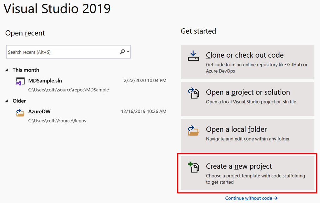
   Figure 4.1 – Creating a new project in Visual Studio

2. Choose Analysis Services Multidimensional and Data Mining Project and click Next:
   

   Figure 4.2 – Creating an SSAS multidimensional project

3. You now are ready to Configure your new project. You will be asked to fill in the following properties associated with your project:

   a) Project Name: WideWorldImportersMD

   b) Location: This will be the location where you want to store the project

   c) Solution Name: WideWorldImportersSSAS

   Naming your Visual Studio project and solution

   There are a couple of comments to be made on the names. We can put this project and the tabular project we'll create later into the same solution. This will simplify the process as we can add a project in later sections.

4. Click Create when you are done.

Congratulations! With that, you have created the project. If you are new to Visual Studio, now is a good time to review the integrated development environment (IDE). When you have a new project, the two key features you need to know about are the design surface and the Solution Explorer. In the following screenshot, we have highlighted the design surface (1) and the solution explorer (2):

Figure 4.3 – Blank canvas for a new project in Visual Studio 2019

As we continue the process of getting the project ready so that we can build out our first cube, we will be working with the solution explorer, which will add tabs or pages to the design surface.

The next few sections will cover the base items that will support the entire project. First, we will create the connection to the WideWorldImportersDW database that we created. Then, we will create the data model, which will be the basis for cube development.

Adding the SQL Server database connection to the project

SQL Server Analysis Services (SSAS) supports connecting to many different data systems. For our hands-on example, we will be connecting to SQL Server 2019 and the WideWorldImportersDW database.

Database connections are created in the Data Sources section of Solution Explorer. Let's get started:

1. Right-click on the Data Sources folder in Solution Explorer. This will open a menu where you can choose to create a New Data Source…, as shown in the following screenshot:
   

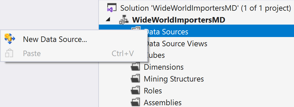
   Figure 4.4 – Creating a new data source from the Solution Explorer

2. Click New Data Sources… to open the Data Source Wizard screen.
3. Click Next on the screen that appears.
4. On the next screen, select How to define the connection and change the selection to Create a data source based on an existing or new connection. Then, click the newly exposed New button. This opens the Connection Manager screen.
5. Set the following Connection properties on the Connection Manager screen:

   a) Provider: Choose Native OLEDBSQL Server Native Client 11.0.

   b) Server Name: Enter your server name here.

   c) Authentication: I am using Windows authentication. However, you may need to use SQL authentication and the username and password if you have issues with Windows authentication. You can use the username and password you created when installing SQL Server in Chapter 1, Analysis Services in SQL Server 2019. This is not an uncommon experience when performing local development with SSAS.

   d) Connect to a Database: You can either select the WideWorldImportersDW database from the list or type it in. Either option works.

6. We recommend that you click the Test Connection button to verify that the authentication works and that the connection is good. Click OK after testing the connection.
7. Now, you should be back in the connection wizard with your newly created connection in the Data Connections list already selected. If it is not selected, select it now.

   What if you have more connections in your list?

   It is possible to have more connections show up in your Data Connections list. This usually occurs if you have other Visual Studio projects that have used similar connection processes. Be sure to connect the connection to the WideWorldImportersDW database before proceeding.

8. Once you have selected the correct connection, click Next.
9. You should now be on the Impersonation Information dialog of the Data Source Wizard screen. This allows you to select the authentication options you will use when loading data into the SSAS database once it has been built. For our purposes, select Use the credentials of the current user. This is useful for the local development and deployment we will be using. However, other options are better choices for production deployments. The option you choose for a production deployment will depend on the security and authentication methods that have been implemented within your organization.
10. Give the data source a name (the default is fine) and click Finish.

Congratulations! With that, you have created the data source. This is now in the Data Sources folder. Now, we are ready to create our data source view.

Adding the DSVs to the project

Data source views (DSVs) serve as the translation layer between the source of your data and the SSAS model. In Chapter 3, Preparing Your Data for Multidimensional Models, we created views in the database to serve in a similar capacity. Why both?

DSVs in SSAS serve as an abstraction layer from the underlying data source. This means that data not in a DSV cannot be accessed by the multidimensional model. If you want to use the data for design, it has to exist in the DSV.

Database schemas and security

In the previous chapter, we created a schema and added the views that will support our model build. It is a good practice to use a specific user or system account in production deployments. When combined, these two activities limit access to the schema and data for the model. If you implement this during design, you can create an Active Directory group and give it permissions to the schema. This will limit access to data for developers as well.

DSVs become more important when the multidimensional model designer has no access or influence on the underlying database. As an example, multidimensional models are often created to make data in data warehouses more accessible. This includes non-Microsoft database systems such as Oracle.

In situations where the data warehouse team and the business intelligence team are not the same, multidimensional model development can be significantly hindered if database views cannot be easily created. In a case such as this, a DSV can help with the process. It allows you to add the table and then make changes to support the multidimensional model design.

As we work through this section, we will be creating our core DSV based on the Cube schema we created in Chapter 3, Preparing Your Data for Multidimensional Models. However, we will also add a couple of tables using the DSV directly with the tables. We will then illustrate some changes that can be made in the DSV, such as using a relational view.

Creating DSVs from relational views

The following steps will help you create a DSV from the Cube.Customer view in the Cube schema. Let's get started:

1. Right-click the Data Source Views folder in Solution Explorer and select New Data Source View… to open the respective wizard, as shown in the following screenshot:
   

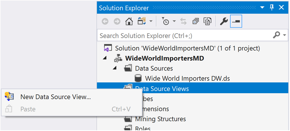
   Figure 4.5 – Creating a new data source view

2. From the welcome screen, click Next to get started.
3. In the Select a Data Source dialog, you can select an existing data source or create a new one. We created the data source in the previous section, so it should be in the list of Relational data sources. Select the data source you created in the previous section and click Next.
4. The Select Tables and Views dialog lists the available tables and views you can add to your DSV. In the Available objects list, you can see all the tables and views you have access to from the data source. If you have implemented security for your developers, which limits the schemas or objects they can see, this will be similarly filtered. Also, you are unable to select any other types of database objects. The list is limited to tables and views. The schema name is in parenthesis after the table or view name.
5. You should also see a Filter field, which is located under the Available objects list. This feature is particularly helpful when working with large lists of tables and views. It filters for the word or words listed there. Try it out using cube to see the list become limited to those items in the Cube schema.
6. You can move the entire list of remaining objects to the Included objects list by clicking the >> button between the lists. You can also move objects one at a time using the > button or remove them from the Included objects list using either << for all selected or < for one at a time. If you are following along, your wizard dialog should look as follows:
   

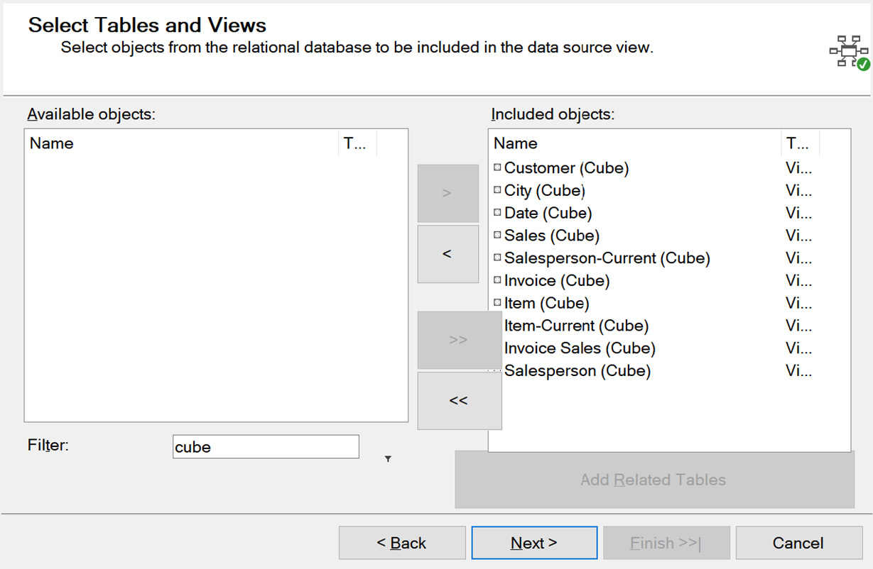
   Figure 4.6 – Select Tables and Views window

   Adding related tables to the Data Source View Wizard

   The option to Add Related Tables is the button below the Included objects list. This button will add all the tables related to the table you add. For example, if we selected the Sales (Fact) table and then clicked the Add Related Tables button, it would add the Employee (Dimension), Customer (Dimension), Date (Dimension), Stock Item (Dimension), and City (Dimension) tables to the Included objects list. This does not work when using relational views. While it can be inconvenient to use relational views, using views is still a better practice in most cases. We do not recommend trading development convenience for maintainability.

7. Once you have moved all the Cube schema objects to the list of Included objects, click Next.
8. Give your DSV a name. The default name uses the same name as the data source. This is fine for our use, but feel free to change it to something that means more to you. Once you've done this, click Finish to close the wizard.

Double-click the DSV you just created to open the Design view for the DSV. As shown in the following screenshot, we do not have any relationships between our tables. This is what we will look at next:

Figure 4.7 – DSV Design view before relationships

We will be adding diagrams for each fact table we included. The diagrams help us keep the views organized around themes. We will also add relationships to finalize our DSVs for the next steps.

Before we start the next section, let's do a quick refresher on our data model. We have created eight dimensions, two of which are current. We have also created two fact tables. The Sales fact view matches the Fact.Sale table in the data warehouse and the data is at the line item level. The Invoice Sales fact view aggregates the date in Fact.Sale to the invoice number level. Therefore, we will create two diagrams that have some dimension table overlap – Sales Diagram and Invoice Sales Diagram.

Creating the Sales diagram and its relationships

1. Create a new diagram by right-clicking on Diagram Organizer in the top-left corner of the DSV Design window. Click New Diagram, name it Sales Diagram, and hit Enter.
2. You will now have a blank diagram window. We will now drag the tables we want to include in this diagram. Let's start by dragging the Sales table onto the diagram design surface.
3. Next, we'll add the dimensions we want to include; that is, City, Customer, Date, Item, Item-Current, Salesperson, and Salesperson-Current. When you drag them in, place them around the Sales table, as shown in the following screenshot:
   

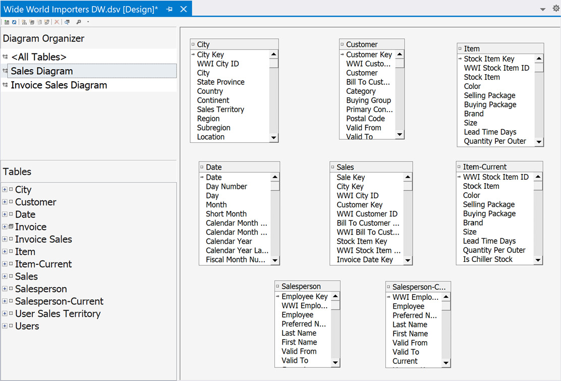
   Figure 4.8 – Sales diagram with dimension tables

4. You can create relationships in the diagram in two ways:

   a) The first way is to drag the column from the Sales table and drop it on the matching column in the dimension table. For example, you can drag City Key from Sales to City Key on City.

   b) The other option is to right-click the Sales table and choose New Relationship.

   Both of these techniques will open the Specify Relationship dialog. If you drag and drop the column, the columns will be filled in. In that dialog, you can update the source and destination tables that will be used in the relationship. The Source (foreign key) table is the fact table. In our case, select Sales from the drop-down list. The Destination (primary key) table is the dimension table. In this case, select City from the drop-down list.

5. For both Source Columns and Destination Columns, choose City Key. This will build the relationship between the two tables. If you have the source and destination tables in the wrong order, an error will occur. You can use the Reverse button to switch the tables so that they're in the correct relationship direction. Once you've done this, click OK. You should see the following output when this step is complete:

Figure 4.9 – Relationship created between Sales and City

To complete this diagram, repeat the previous process and create the remaining relationships. Use the following list to create the remaining relationships. The first two lists are followed by the action to be taken after they are created. The list is organized as follows: Source table, key field > Destination table, key field. Here is the first list:

• Sales, Customer Key > Customer, Customer Key
• Sales, Stock Item Key > Item, Stock Item Key
• Sales, WWI Stock Item ID > Item-Current, WWI Stock Item ID

When creating this relationship, you may be prompted to create a Logical Primary Key in the Item-Current table. Agree to this change by clicking Yes in the dialog that opens as follows:

Figure 4.10 – Prompt to create a logical primary key in your DSV

Here is the second list:

• Sales, Salesperson Key > Salesperson, Employee Key
• Sales, WWI Employee ID > Salesperson-Current, WWI Employee ID

When creating this relationship, you will be prompted to create a Logical Primary Key in the Salesperson-Current table. Agree to this change by clicking Yes in the dialog that opens.

Here is the third list:

• Sales, Invoice Date Key > Date, Date
• Sales, Delivery Date Key > Date, Date

  Role-playing dimensions

  A role-playing dimension is a dimension that has multiple relationships with the fact table. From a data warehouse implementation, it is more space-efficient to create separate relationships from the same table. In our design, the date is used for Invoice Date and Delivery Date, which have distinct relationships but use the same dimensional data. This type of relationship happens often in a data warehouse.

Now that the relationships have been created, your Sales diagram is complete. It should look as follows:

Figure 4.11 – Completed Sales diagram in the DSV

Next, we'll create a diagram for Invoice Sales and its relationships.

Creating the Invoice Sales diagram and its relationships

Next, we need to create the Invoice Sales diagram. This process is similar to the one we followed for the Sales diagram. Here is the list of relationships you will need to complete. The following list contains Source table, key field > Destination table, key field:

• Invoice Sales, Customer Key > Customer, Customer Key
• Invoice Sales, City Key > City, City Key
• Invoice Sales, Salesperson Key > Salesperson, Employee Key
• Invoice Sales, WWI Employee ID > Salesperson-Current, WWI Employee ID
• Invoice Sales, Invoice Date Key > Date, Date
• Invoice Sales, WWI Invoice ID > Invoice, WWI Invoice ID

The resulting Invoice Sales diagram should look as follows:

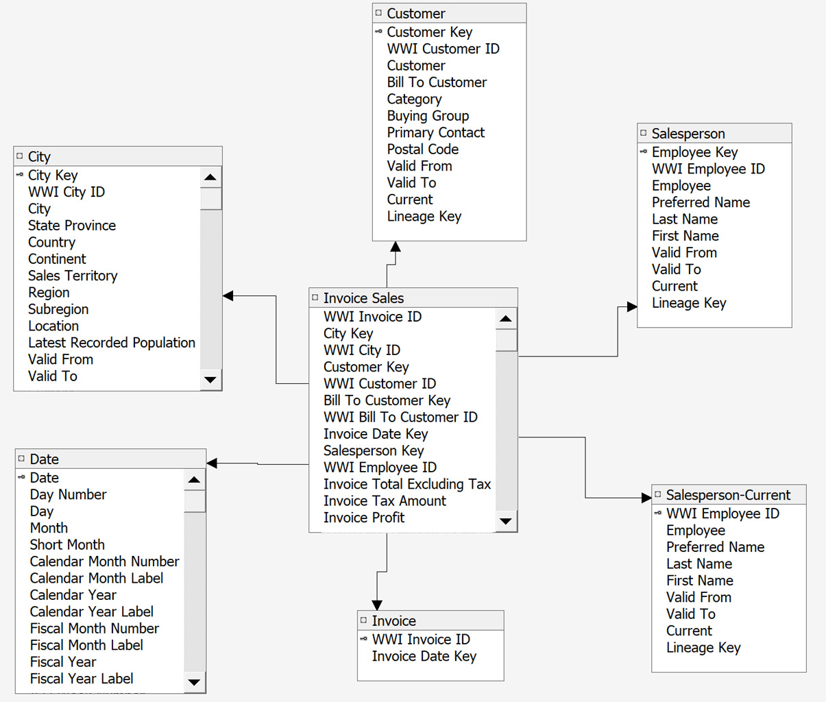
Figure 4.12 – Completed Invoice Sales diagram

We will now review the DSVs.

Custom DSVs

Before we move on to building out the dimensions and measure groups, we need to review some additional capabilities available in our DSVs. We are going to update an existing table and add some additional fields to it. To do this, we will replace the table with a New Named Query. Let's get started:

1. Open the Data Source View Design window.
2. Right-click on the Invoice table name in the Tables panel. Here, you'll see the Replace Table option. Expand that menu and choose the With New Named Query … option, as shown in the following screenshot:
   

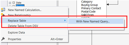
   Figure 4.13 – Creating a new named query to replace an existing table

3. This will open the Create Named Query dialog. We will be changing the SQL section at the bottom. This is highlighted in the following screenshot:
   

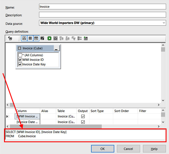
   Figure 4.14 – Create Named Query dialog with the SQL section highlighted

4. Replace the query in the dialog with the following code:

   SELECT [WWI Invoice ID]

   , [Invoice Date Key] as [Invoice Date]

   , CAST(DATEPART(year, [Invoice Date Key]) AS VARCHAR) + '-'

       + CAST(DATEPART(month, [Invoice Date Key]) AS VARCHAR) AS [Invoice Month]

   , DATEPART(year, [Invoice Date Key]) AS [Invoice Year]

   FROM Cube.Invoice

5. Click the green Run button in the Query definition section to update the query. This should return the rows and update the dialog. When you can run this without errors, click OK to close the dialog.
6. You will now see the additional fields in the DSV model. Because we did not change the key column and we replaced the existing Invoice table, the relationships stayed intact.

Now that we have created the Data Source View, we can start adding dimensions.

Adding dimensions, attributes, and hierarchies

In SSAS, dimensions are comprised of a group of attributes and hierarchies that define the dimension. Before we get into how, we need to discuss three key topics; that is, dimensions, attributes, and hierarchies:

• Dimensions are the slicers we use in our cubes to filter and segment our data for analysis. We defined our dimensions in Chapter 3, Preparing Your Data for Multidimensional Models.
• Attributes are the various related items in our dimension. For example, if we use the City dimension, the attributes include City Name, City Key, Country, State or Province, and Last Recorded Population. These are the fields we added to our DSV.
• Hierarchies help us organize our attributes. A hierarchy gives us a clear drill path into our data. In our City dimension, we will create a Geography hierarchy that consists of Country, State or Province, and City in that order. The goal of hierarchies is to be able move through our data in a well-understood fashion.

Now is a good time to remind you that multidimensional databases have been around for many years. As a result, they have been modified significantly and have a wealth of capabilities that are outside the scope of this book.

In the next few sections, we will create our dimensions through the use of the Dimension Wizard window. This is the most efficient method to do this. Once the dimensions have been created, we will create the hierarchies and attribute relationships. This is the most basic development task required to create dimensions. The remaining sections will call out specific, more advanced techniques that can be used improve the usability and performance of the dimensions. Let's get started.

Creating dimensions with the Dimension Wizard

Let's begin with creating dimensions with the dimension wizard with the help of the following steps:

1. The first step is to make sure we have the project open and can see the Solution Explorer window. Right-click the Dimensions folder in your Analysis Services project. You will see the option for New Dimension…, as shown in the following screenshot. Click that to launch the wizard:
   

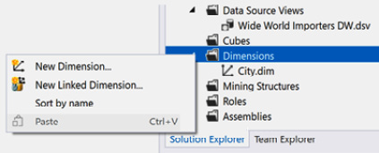
   Figure 4.15 – Launching the Dimension Wizard from Solution Explorer

2. Now that you have the Dimension Wizard window open, you can click Next to move to the first action screen – Select Creation Method.
3. You will see a list of options for creating dimensions. Because we are using a full data warehouse and we have created our DSV, we will use the default option; that is, Use an existing table. With that selected, click Next.

   Other dimension creation methods

   As shown on the Select Creation Method screen of the Dimension Wizard window, you can create dimensions by generating tables. Two of the options are designed for situations when you need a Date dimension by generating a table in the DSV or underlying data source. While convenient, we typically recommend against this process. The reason for this is that most of the time the wizard does not generate the attributes you need in your model. Most data warehouses, such as ours, have a date dimension created to support this functionality. The third option uses a generic template to create dimension tables. For example, you can create a customer dimension using the Customer Template option. However, you will still need data to support this. If you are looking for design examples for various business needs, this may be a good way to experiment. Typically, you will follow the pattern we have been using and create a relational star schema to support multidimensional model design.

4. In Specify Source Information, select Data source view, Main table, and Key columns. For our first run with the wizard, we will select Customer for our main table. You will see that if keys are defined in the DSV, they will populate the Key columns section. Confirm that Customer Key is listed in the Key columns section and then click Next.
5. Next, we'll select the attributes we want to include in our dimension. This page lists all of the attributes or fields from the Customer table in the DSV. You have three options for each attribute. By selecting Attribute name, you are choosing to include it in the dimension. The next option is Enable browsing. This option will set the property that makes the attribute available in client tools. Finally, you can choose an Attribute type. The next few steps will walk through these in detail.

   Choosing your dimension attributes

   Every field can be chosen as an attribute. Here are some of the key considerations when choosing an attribute:

   a) Does the business need the attribute? System values are typically not necessary for development. Examples commonly include lineage IDs and other fields designed to support the load process.

   b) Is the field used at all? Just because the name sounds good does not mean it is a candidate for an attribute.

   c) The primary consideration is that the attribute needs to have value to the business or is necessary for a calculation. Don't include the attribute just because it is there.

6. We will use all the attributes except Valid From, Valid To, Current, and Lineage Key. This will be a common practice for all our dimensions as we build them. For the customer dimension, leave Enable browsing selected. We do not need to change our Attribute type. Your screen should look as follows:
   

   Figure 4.16 – Customer Dimension Wizard with attributes selected

7. Click Next to preview the dimension. If everything looks correct, click Finish to close the wizard and create the Customer dimension.

Congratulations! You have created the first dimension in your multidimensional model. You should now see the Design tab for your dimension open in Visual Studio. Now, we need to add our remaining dimensions. For each of the dimensions, you will go through similar steps to what we followed here. We have listed each dimension here, along with any changes you should consider while creating them:

• City: The wizard does not have Enable browsing selected for Location. Location is a geography data type that is not supported in SSAS. We recommend that you do not include that attribute. In the Attribute type section, you will see that there is a Geography list of types. Go ahead and set Attribute type for City, State Province (State or Province), Country, and Continent. You should also set the dimension as a Geography type. This increases support in visualization tools.
• Item: No changes from the pattern are required for this dimension.
• Current Item: We are changing the name of this dimension, which is based on Item-Current in the last step to Current Item. This will be more understandable for our users.
• Salesperson: We are using the Salesperson-Current table for this dimension, not the Salesperson table. There are changes to the Salesperson dimension that we need to bring into the multidimensional model, which means we will have only one Salesperson dimension in use.
• Invoice: Change the name of WWI Invoice ID to Invoice Number. This can be done on the Selection Dimension Attributes page of the wizard by double-clicking the WWI Invoice ID name.
• Date: Date needs to have its Attribute types set. When you click the dropdown list, you will find Date, which expands into date categories and specific types for those categories, as shown in the following screenshot:
  


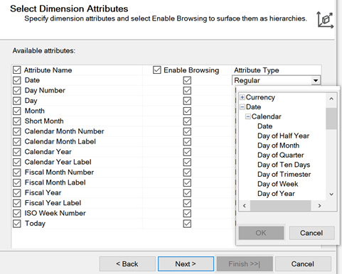
Figure 4.17 – Selecting attribute types for the Date dimension attributes

Here is the completed dialog box for your reference. You will also find attribute types for the standard calendar dates, fiscal dates, and ISO:

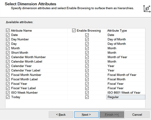
Figure 4.18 – Completed attribute types for the Date dimension attributes

You should see all your dimensions in the Dimensions folder in Solution Explorer. You should also have all the dimension Design tabs open in Visual Studio.

Using the Business Intelligence Wizard to set attribute types

We could have used the Business Intelligence Wizard on both the City and Date dimensions to set the attributes. The Business Intelligence Wizard is designed to support tasks such as attribute types. Because we did this while creating the dimension, it is not necessary. If you want to view the wizard, right-click the Date dimension and choose Add Business Intelligence. Select Define Dimension Intelligence to view the mapping you just completed. This works with the City dimension as well. This is just one other option you can use to set the attribute types for your dimension.

Combining the key and name attributes

Before we start working on the hierarchies, we need to combine the dimension key with its name. This is important as we do not need the surrogate key available in the hierarchy or to users as it is meaningless. This process will result in the name or other meaningful attributes being visible to the users while the data is optimized using the key in the background. Let's begin:

1. Go to or open the City dimension Design page.
2. Click on the City attribute in the Attributes pane.
3. In the Properties pane, find the Source section and change KeyColumns from City.City to City.City Key. When you choose to change this, the Key Columns dialog will open. In that dialog, remove the City column first, and then add the City Key attribute. This will result in City.City Key (Integer) being in the property.
4. Change NameColumn to City.City (WChar).
5. Find the Usage property in the Basic section and change it from Regular to Key.
6. Delete the City Key attribute from the Attributes pane.

This will set the City attribute as the key column for the City dimension. We have highlighted the areas you need to be concerned with in the following screenshot:

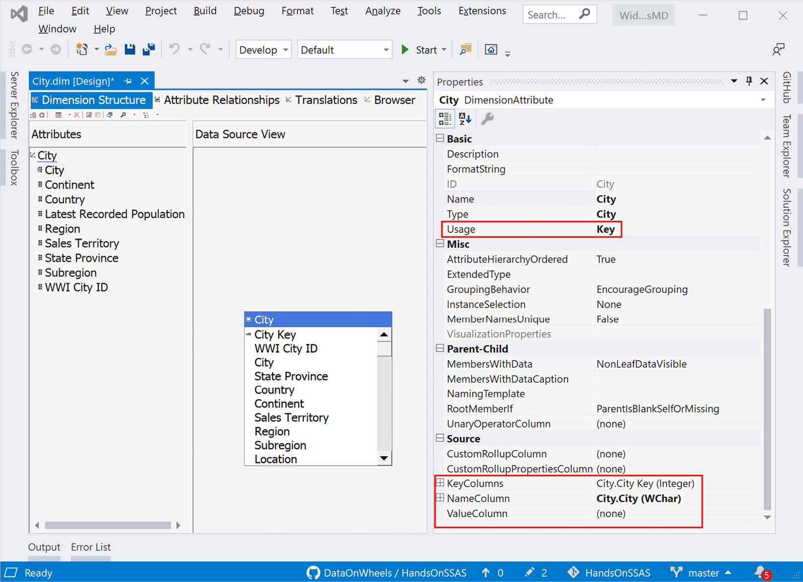
Figure 4.19 – Changing the dimension key

This process should be completed for each dimension, before you add the hierarchies. The following is the list of keys and names for the remaining dimensions that need to be modified (not all the dimensions need this update):

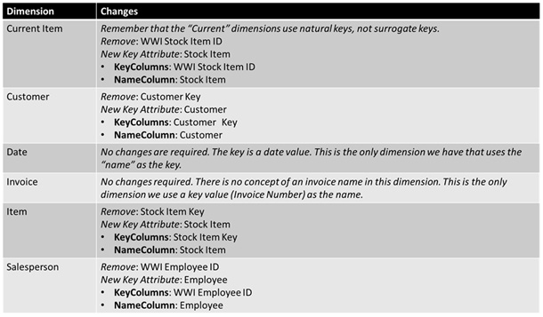
Figure 4.20 – Dimension and hierarchy definitions

Reminder

Be sure to save your work on a regular basis.

Adding hierarchies to your dimensions

Hierarchies are key to good design in all business intelligence models. However, in multidimensional models in SSAS, they are even more important. They enhance the user experience, improve performance, define aggregation levels, and refine storage patterns for the data.

Let's dig into some basics about hierarchies that you should know about. First, we need to differentiate between natural and unnatural or artificial hierarchies:

• A natural hierarchy is a set of attributes in a dimension that are related in a pattern from the smallest to the largest group. For example, a common natural hierarchy is date. We know that a year has four quarters, each quarter has 3 months, and that each month has between 28 and 31 days. The following diagram illustrates the pattern we look for in natural hierarchies:

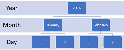
Figure 4.21 – Sample date hierarchy

• An unnatural or artificial hierarchy is when the attributes are not related in a natural pattern and can have inconsistent group sizes throughout. These hierarchies are typically helpful to the business for analysis but are not organized well in the data. A clothing dimension provides a clear example of this type of hierarchy.

The natural hierarchy might contain Type (outdoor, indoor), Style, and Product or the item of clothing. However, the business may want to create an artificial hierarchy using different attributes, such as Color and Size. The business now wants a hierarchy that uses the following pattern: Season, Style, Color, Size. The following diagram illustrates the imbalance between natural and artificial hierarchies based on the data:

Figure 4.22 – Unnatural or artificial hierarchy of clothing

This is not ideal as it cannot be optimized for SSAS. While it is possible to create these in SSAS, it is typically not recommended. This is particularly true now that tools such as Power BI can handle those requirements easier in their design tools. We will be creating natural hierarchies in our dimensions in the next section.

Creating and updating attribute hierarchies

Once a dimension has been created, every attribute is created as a two-level hierarchy. The levels are All and the attribute itself. As we discussed previously, this is to support aggregations and storage. When measures are added later, each attribute will be aggregated at the All level and the individual attribute level. In some cases, this is what we want. However, we typically do not deal with most attributes in isolation, which is why we create hierarchies.

We will start with the City dimension. Go to the Design tab for the City dimension. If you have closed your tabs or Visual Studio, reopen the project, expand the Dimensions folder, and double-click the City dimension to reopen the Design tab. You should be looking at a screen similar to the one shown here:

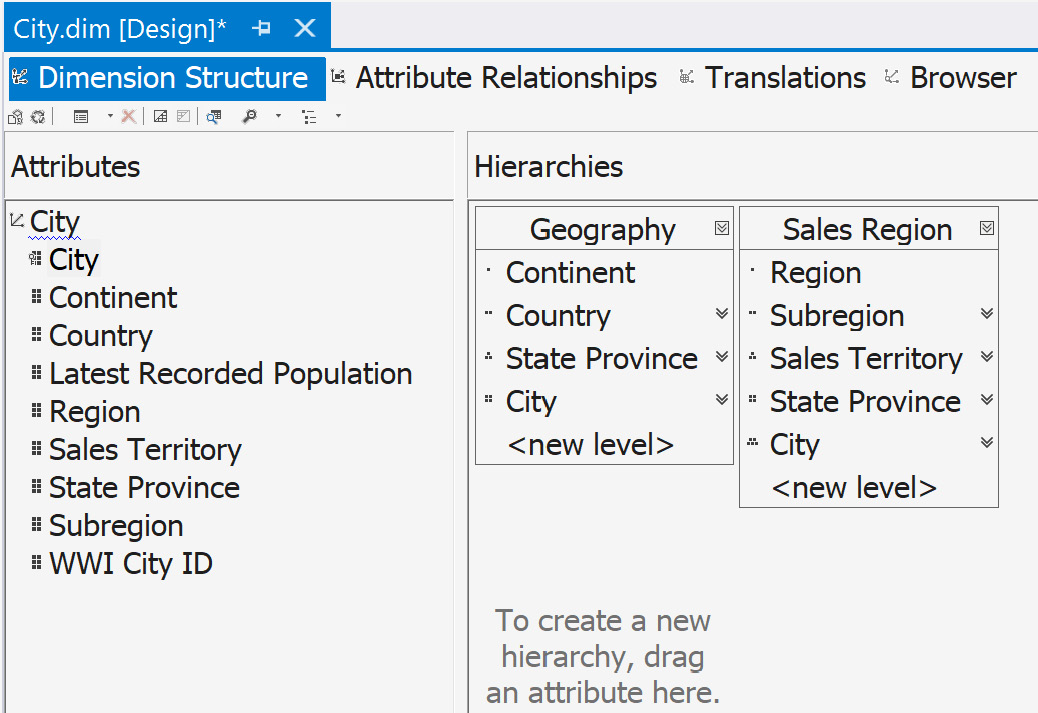
Figure 4.23 – Dimension design window with the Attributes and Hierarchies panes highlighted

We will be working with the Attributes and Hierarchies panes to create our hierarchies. Typically, we should know the hierarchy options through data or business analysis. In this case, we will be creating two hierarchies:

• Geography: This hierarchy will have a standard pattern for supporting continents to cities.
• Sales Region: This hierarchy will support the sales territories as defined by Wide World Importers.

We will create each hierarchy using the following steps:

1. We will start with the Geography hierarchy. Drag the Continent attribute onto the Hierarchies pane. This will create a new hierarchy with Continent as the first level.
2. Rename the hierarchy Geography. You can do this by clicking Hierarchy in the new hierarchy table or by changing the name in the Properties window, which can usually be found on the right-hand side of the screen, under Solution Explorer.
3. Next, drag the Country and State Province attributes onto the hierarchy you just created in that order. You should target the <new level> row in the Geography hierarchy. Don't worry if you drop it in the wrong place; you can move the levels around by dragging them up or down as needed.
4. Finally, add the City attribute as the lowest level. As the key or leaf level, this is where the relationship will be made with the fact table, as defined in the DSV.
5. Now that the Geography hierarchy is complete, we can create the Sales Region hierarchy by dragging the Region attribute onto an empty area of the Hierarchies pane.
6. As we did previously, rename the hierarchy by clicking into the header and giving it the name Sales Region.
7. The rest of the attributes to add are Subregion, Sales Territory, State Province, and City in that order.

Staying in the City dimension, you might have seen the warnings in the hierarchies letting you know that the attribute relationships are not in place. That is the next area of focus for our dimension build-out.

Adding attribute relationships

Attribute relationships in SSAS support additional query and storage optimizations. SSAS uses the defined relationships to consolidate processing operations, which makes loading data into a multidimensional model (processing) and querying data in the model more efficient. SSAS optimizes storage by using more compression when attribute relationships are defined.

When we created the hierarchies, SSAS assumed that the relationships could be optimized based on the relationships in the hierarchies. Let's add the relationships that support the hierarchies we have created.

When you open the Attribute Relationships tab on the City dimension's Design window, you will see that all the attributes that have been added to our hierarchies have been mapped to City. The remaining attributes are considered direct attributes that have a 1:1 relationship with City:

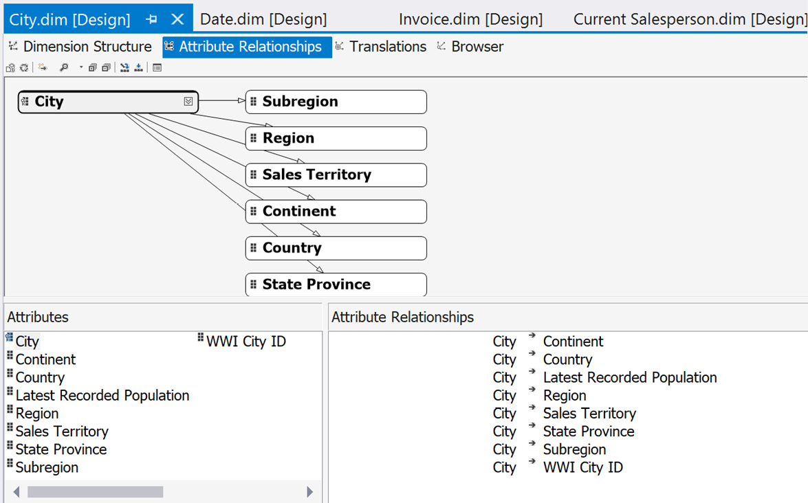
Figure 4.24 – City dimension attribute relationships before applying hierarchy mappings

You can change the mapping in a couple of ways. The easiest and sometimes the most frustrating option is to drag and drop. You can create the relationship between Country and State Province by dragging State Province onto Country. The resulting relationship is State Province > Country. If you do this the other way around, you will need to fix the relationship. You can also adjust or create the relationship by right-clicking on the attribute relationship in the pane on the right, under the mapping window. This will open the following dialog, where you can add or create the relationship you need:

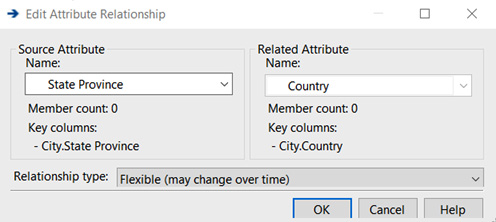
Figure 4.25 – Edit Attribute Relationship dialog

Whichever pattern you choose, you should end up with a set of relationships that match the hierarchies we created.

Flexible versus Rigid attribute relationships

The default type of relationship for attributes is Flexible, which assumes that the relationship could change over time. This is the default and most flexible option, as the name suggests. However, this is less efficient if Rigid is a valid option. Rigid assumes the relationship will not change over time. A great example of a Rigid relationship is in the Date dimension. Years have quarters, quarters have months, and months have days. This will not change. However, an employee dimension could see people promoted to managers. This would require the Flexible relationship type to support the movement of attributes and their relationship over time. Be aware that if you choose Rigid and a change does occur, the model load may fail as a result.

Here is what the attribute relationships should look like when they are mapped correctly:

Figure 4.26 – City dimension attribute relationship configured correctly

Building out the rest of the hierarchies

You need to have followed the preceding steps for each of the dimensions we have created. Let's take a look at the hierarchy definitions for each of the remaining dimensions. Remember to create the hierarchy and then update the attribute relationships for each of these dimensions. We have included the attribute relationship image for each dimension as a reference.

Hierarchy and dimension names must be unique in the multidimensional model

When designing a multidimensional model, it is common to have names repeated in the design. When working with hierarchies and dimensions, your hierarchy names need to be unique within the model; otherwise, you will get a build error. For example, the Current Item and Item dimensions have the same structure, while the Brand hierarchy we are creating will need to be named differently to prevent conflicts. We will also use Customer Hierarchy in the Customer dimension to differentiate the hierarchy from the dimension.

Here is the attribute relationship for the Current Item and Item dimensions:

• Current Item dimension:

  Hierarchy Name: Current Item Brand

  Hierarchy Levels: Brand > Stock Item

• Item dimension:

  Hierarchy Name: Item Brand

  Hierarchy Levels: Brand > Stock Item:

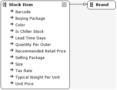
Figure 4.27 – Current item and item dimensions attribute relationships

Here is the attribute relationship for the Customer dimension:

• Customer dimension:

  Hierarchy Name: Customer Hierarchy

  Hierarchy Levels: Category > Buying Group > Bill To Customer > Customer:

Figure 4.28 – Customer attribute relationships

Here is the attribute relationship for the Date dimension:

• Date dimension:

  Hierarchy Name: Calendar

  Hierarchy Levels: Calendar Year (Calendar Year Label attribute renamed Calendar Year) > Calendar Month (Calendar Month Label attribute renamed Calendar Month in the hierarchy) > Date

  Hierarchy Name: Fiscal

  Hierarchy Levels: Fiscal Year (Fiscal Year Label) attribute renamed Fiscal Year in the hierarchy) > Fiscal Month (Fiscal Month Label attribute renamed Fiscal Month in the hierarchy) > Date

  Hierarchy Name: ISO Week

  Hierarchy Levels: ISO Week Number > Date:

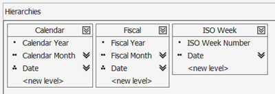
Figure 4.29 – Date dimension hierarchies

Once you've created the hierarchies, you should set the relationships up like so:

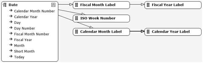
Figure 4.30 – Date dimension attribute relationships

Here is the attribute relationship for the Invoice dimension:

• Invoice dimension:

  Hierarchy Name: Invoice Hierarchy

  Hierarchy Levels: Invoice Year > Invoice Month > Invoice Date > Invoice Number:

Figure 4.31 – Invoice dimension attribute relationships

Here is the attribute relationship for the Salesperson dimension:

• Salesperson dimension – no hierarchies or updates to attribute relationships required

Now that we have all the dimensions built, along with their hierarchies, we can load and preview the data. The next section describes how you can process your dimensions, which will load the data into SQL Server 2019 Analysis Services.

Processing the dimensions

Processing in SSAS multidimensional models is the method of loading the data into the multidimensional database. At the end of this chapter, we will dive into processing techniques in more detail. The focus of this section is processing our dimensions. We will walk through processing the City dimension in this section. By doing this, you will be able to apply these steps once more so that you can process the rest of the dimensions. Some of the setup here is for the entire project and will be repeated in the processing section at the end as well.

Prepping your project for processing

The following steps only need to be done if you have not already set up the deployment properties for your project. For these steps to work, SSAS in multidimensional mode should be running:

1. Right-click on the project name in Solution Explorer and select Properties from the menu.
2. This will open Property Pages for the project. You will see the Configurations Properties page and three sections called Build, Debugging, and Deployment.
3. In the Build section, set Deployment Server Edition to Developer.
4. In the Deployment section, set Server Name to the server you have running in multidimensional mode. In most cases, Localhost, the default option, will not be correct if you set your environment up with named instances, as recommended in Chapter 1, Analysis Services in SQL Server 2019.
5. Click OK to apply these changes.

   Your project should now be ready to deploy to Analysis Services. Let's take a look:

6. Right-click on the City dimension and select Process….
7. This step only applies if you have made changes to the project since the last time it was processed. You will see a message that states The server content appears to be out of date. Would you like to build and deploy the project first?. Select Yes to continue with the build and deployment.
8. Once the project changes have been built and deployed, you will see a Process Dimension dialog box. We will spend more time on processing options later in this chapter. For this section, leave the default settings as is and click Run to continue.
9. Once this has completed, you can close all the open windows.
10. Now, go to the Browser tab in the City dimension's Design tab to explore the hierarchies you've created. You will also see the other hierarchies, which are single levels under the All level.

Solving impersonation issues while processing

One of the most common and annoying issues with SSAS in a development, non-enterprise network environment is due to impersonation. You may recall when we created the data source at the beginning of this chapter that we used Use the credentials of the current user for impersonation. This impersonation has served us well for development and my work for you as well.

In my setup, this did not work when processing because the current user is the SSAS NT Service account, which is running the service. This is a default service that was user created when my account was set up. To work around this issue, I added that user account to my WideWorldImportersDW database in the db_datareader role. If you have issues with processing, you can use this option. I would not recommend this for production use. A system account with the appropriate permissions should be used to manage this scenario. We will discuss this in detail in Chapter 11, Securing Your SSAS Models. If you want to implement the solution I used quickly, run the following scripts in SQL Server Management Studio when it's connected to your SQL Server Data Engine instance.

First, you will need get your service account name from our Services console or SQL Server 2019 Configuration Manager. In my case, the account name is NT ServiceMSOLAP$DOWSQL2019. Here are the scripts you need in order to add this user to your data warehouse:

USE [master]

GO

CREATE LOGIN [NT SERVICEMSOLAP$DOWSQL2019] FROM WINDOWS WITH DEFAULT_DATABASE=[master], DEFAULT_LANGUAGE=[us_english]

GO

USE [WideWorldImportersDW]

GO

CREATE USER [SSASMDSys] FOR LOGIN [NT SERVICEMSOLAP$DOWSQL2019]

GO

USE [WideWorldImportersDW]

GO

ALTER ROLE [db_datareader] ADD MEMBER [SSASMDSys]

GO

Depending on your environment setup, this option may not work. In some cases, using a Windows account may work. These issues typically affect development environments that are not connected to an Active Directory domain. If you are connected to a domain, service accounts will support a more cohesive solution.

Processing the rest of the project

Now that we have successfully processed the City dimension, you can choose to process everything we have created so far by right-clicking the project name and selecting Process All. This will confirm everything is working. If you have any errors, fix them and process everything again. You can also choose to process them one at a time so that you can deal with issues on a smaller scale. You must remember that the process queries the source database and replaces the data with new data. When working with larger multidimensional models, this can be a time issue. If your development environment is not very powerful, you could even experience issues with our project.

Whether you process the entire database or one object at a time, a processing log is displayed at the end. This provides the processing time and row counts for all the dimension attributes and hierarchies that have been processed. You should take a moment to explore the log to see the details of the work you have done. You should also browse the dimensions to see how the data will be presented in end user tools. This is an excellent way to handle issues early in the design process.

Updating our dimensions

If you have taken the time to browse the data, you may have noticed some issues with our dimensions. The obvious issue is ordering dates. We would like them ordered by date, not name or label. We will fix that order in this section, as well as the order for the Salesperson dimension.

Another issue is with the Customer dimension. Bill To Customer and Customer have duplicate values in the Customer hierarchy for the head office of both Tailspin Toys and Wingtip Toys. These are the two customers that are currently available in our data. We will implement ragged hierarchy principles here to hide duplicate values. Let's get started with fixing the sort order in our dimensions.

Fixing dimension and hierarchy orders

By default, dimension and hierarchy attributes are sorted by the key in the attribute. You can sort attributes by other attributes in the dimension. Let's fix one so that you have an example to work with. We will start with the Date dimension. SSAS knows how to sort dates properly, so the lowest level, Date, is sorted correctly. However, we need to fix the Month levels. Both the Fiscal and Calendar hierarchies have issues with the Month level sorting. The Year and Date levels are fine. Let's get started:

1. Open the Date dimension's Design window.
2. Click on the Calendar Month Label attribute in the Attributes panel. This is the attribute that's used in the Calendar Hierarchy Calendar Month level.
3. In the Properties panel, we need to add Calendar Month Label to the NameColumn property.
4. Next, we need to add the Calendar Month Number attribute to KeyColumns. In this dialog, Calendar Month Number needs to be on top of the list. This effectively makes the key a combination of both.
5. In the Properties panel, find the OrderBy property. OrderBy should be set to Key.
6. Process the dimension and browse the change. (You may need to click the Reconnect button at the top of the Browser window to refresh your results.)
7. Repeat this process for the Fiscal Month Label attribute.

We can also change our Item and Salesperson dimensions so that they use Name instead of Key for the sort order. Let's walk through changing the Salesperson dimension:

1. Open the Salesperson dimension's Design window.
2. Select the Employee attribute in the Attributes panel.
3. In the Properties panel, locate the OrderBy property.
4. Change this from Key to Name. Salesperson will now be sorted by Employee (which is the full name) instead of the WWI Employee ID value that's used in Key.
5. Process the dimension and review the results.
6. Repeat this process with the Current Item and Item dimensions on the Stock Item attribute.

You can apply the same pattern if you have other attributes you would like to change the order of.

Ragged hierarchies

Ragged hierarchies are used when a hierarchy has levels that are skipped or end early. This happens often in geography dimensions, for example. If you have customers in Europe and Canada, you may have different levels of hierarchy.

Let's look at a Canadian hierarchy:

• Country: Canada
• StateOrProvince: Ontario
• City: Dinorwic

Now, let's look at a customer hierarchy in Norway:

• Country: Norway
• StateOrProvince: NONE
• City: Oslo

How is this handled in the data? Often, we repeat the city name in StateOrProvince if it is not in the underlying data or structure. So, Olso would look as follows in the hierarchy:

• Country: Norway
• StateOrProvince: Oslo
• City: Oslo

The issue with this is that no one wants to see this in their report tools. We can remove the second Oslo in the hierarchy by selecting the StateOrProvince level in the hierarchy and changing the HideMemberIf property for the level to OnlyChildWithParentName. This will make the unused level invisible to the report tools.

Let's put this to use with our Customer dimension. We know that head office for both Wingtip Toys and Tailspin Toys is repeated in the Bill To Customer and Customer levels of Customer Hierarchy. Here is how we resolve this issue:

1. Open the Customer dimension's Design window.
2. Select the Customer level in Customer Hierarchy.
3. In the Properties pane for that level, change HideMemberIf from Never to ParentName. This will hide that level when both levels have the same name.

   Impact of ragged hierarchies

   In the geography example, we introduced an artificial level that will have no data associated with it. This means that Oslo levels will return the same values , no matter which level we viewed. However, with our example, data may exist at the Customer level for either head office. This means we will not see the specific order of data for the head offices if it exists. We will leave this in place in our model to demonstrate ragged hierarchies. However, you will need to evaluate the user experience to ensure you display the data as expected to your users.

Using Parent-Child relationships

We do not have an example of Parent-Child relationships in our model. However, as you continue to develop your skills with multidimensional design, you will find that implementing this type of relationship is fairly easy. Two of the most common examples are chart of accounts (general ledgers) and employee reporting structures. Often, that data has an unknown number of levels in it. This results in the underlying table having both a key and a parent key. The following is a partial screenshot of the properties window for a dimension with the various properties that support Parent-Child dimensions:

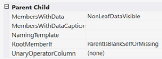
Figure 4.32 – Parent-Child properties

The two key properties to consider are RootMemberIf and MembersWithData. RootMemberIf helps SSAS determine where the top of the hierarchy is. For example, if the top level of your corporate hierarchy is the president and the parent key is null, then you would use ParentIsBlankSelfOrMissing.

MembersWithData helps determine if we display data at intermediate levels. In our previous example, you may have President > Vice President > Director in your hierarchy. You have the option to show data at intermediate levels, which assumes you have data at those levels. In some cases, the only data that matters is at the leaf level. We encourage you to experiment with this property to confirm you have the user experience you need.

One last callout that is unique to multidimensional models is UnaryOperatorColumn. When working with a chart of accounts, the aggregation and signs change as you traverse the hierarchy. For example, expenses are represented as positive numbers until they are at the same level as revenue. Unary operators specify how to aggregate and sign data in the model. This information will have to be part of the dimension table and can be specified here. This is a very powerful implementation and one of the reasons financial analytics are often easier to implement in multidimensional models.

Cleaning up dimension hierarchy lists

We have done a lot of work with our dimensions already. However, there is one more cleanup task we need to implement to make the user experience better for our users. This task involves removing or hiding attributes that are not required in the dimensions.

For example, the Date dimension should only have the hierarchies exposed. As shown in the Dimension Browser tab, all the attributes that are not used in the hierarchy are exposed to the users. This is not a great user experience as those attributes are not very valuable when they're not contained in a hierarchy:

Figure 4.33 – Date dimension hierarchies

You can remove these hierarchies from the list by hiding them. Let's take a look at how to do this:

1. From the Dimension Structures tab, select an Attribute you want to hide.
2. In the Properties pane, find the AttributeHierarchyVisible property and set it to False.

Complete this task for every attribute in the Date dimension you want to hide. We will plan to hide all of them, leaving only the hierarchies we explicitly made visible to users. Hiding these hierarchies only affects the user experience. We can still use these attributes when creating hierarchies or custom calculations.

This concludes our work on dimensions. Next, we will be adding measure groups to see how dimensions slice and dice our data.

Adding cubes and measure groups

In multidimensional models, cubes typically map to fact tables in our data source. They have relationships to all the relevant dimensions and contain measures that can typically be aggregated. Before we dig into creating our cubes and measure groups, let's talk databases and cubes.

In multidimensional models in SSAS, a database generally refers to the overall structure of the SSAS model. When SSAS was first introduced, only one measure group was supported, so the entire structure was referred to the common term cube. As the product matured, the structure became more complex. When we talk about the multidimensional model, we are usually referring to the database. The model or database is made up of dimensions, cubes (which contain multiple measure groups), the DSVs, and data sources. In SSMS, you will see a similar structure to Visual Studio. The project in Visual Studio is the equivalent of the database in SSMS. That being said, cube can also refer to the entire database, even though cubes are specific structures in the model and used by users and developers alike.

Measure groups in SSAS are typically organized around fact tables and share a common set of dimensions. This pattern follows the dimensional model paradigm and is why it is important to have star schemas to support multidimensional models.

Creating the cube and measure groups

In this section, we will create our cube so that it contains our measures. Follow these steps:

1. In Solution Explorer, right-click the Cubes folder and select New Cube… to open the Cube Wizard window.
2. Click Next on the opening screen.
3. Select Use existing tables on the Select Creation Method screen, and then click Next.
4. On the Select Measure Group Tables screen, select the Sales and Invoice Sales tables, and then click Next.
5. On the Select Measures screen, click the Sales and Invoice Sales checkboxes to unselect all the measures.
6. Under Sales, select the following measures to include: Quantity, Unit Price, Tax Rate, Total Excluding Tax, Tax Amount, Profit, Total Including Tax, Total Dry Items, Total Chiller Items, and Sales Count.
7. Under Invoice Sales, select the following measures to include: Invoice Total Excluding Tax, Invoice Tax Amount, Invoice Profit, Invoice Total Including Tax, Invoice Total Dry Items, Invoice Total Chiller Items, Invoice Count, and Sales Count-Invoice Sales.
8. Once the measures have been selected, click Next.
9. On the Select Existing Dimensions screen, select all the dimensions if they have not been selected already. Click Next.
10. On the Select New Dimensions screen, deselect any options here. We do not need to add any suggested dimensions. Click Next.
11. Change the name of the cube to Wide World Importers and click Finish.

You should now see the Wide World Importers Cube's Design window. Congratulations – your first cube with two measure groups has been created! You should see something like the following in your Cube Design window:

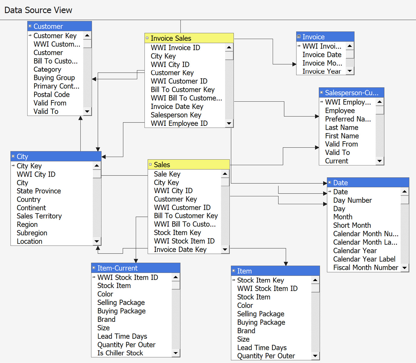
Figure 4.34 – First view of the Cube Design window

The rest of this section will explore the tabs in the Cube Design window. While we may not change each section here, the goal is to make sure you understand their purpose and can implement what you need to deliver specific solutions in your business.

Before moving on to the next section, process the project and resolve any errors.

Reviewing the cube's structure and modifying measures

The specific panes in the Cube Structure tab are Measures, Dimensions, and Data Source View. You can add or modify measures in the Measures pane. If you click a measure, you can review the properties for that measure, including its aggregation, format, and source. In the Dimensions pane, you can add a dimension or go to the Design window for a dimension from that pane. If you need a new dimension or need to remove or add a dimension to the cube structure, you can do that here. The other cube pane is Data Source View. This is the visual diagram of the underlying structure that supports the cube and its measure groups.

Modifying measures

Now, we are going to modify some measures. Cubes present measures based on the settings here. The primary focus will be on the aggregation functions and their formats. Let's modify the Quantity, Total Including Tax, and Tax Rate measures in the Sales measure group. You should update these for each measure in both measure groups before leaving this pane. These examples should help you understand the basics.

Modifying the Quantity measure

The Quantity measure is the quantity of items ordered. We will review the key attributes and add a format string in these steps:

1. Select Quantity under Sales in the Measures panel.
2. In the Properties panel, find AggregationFunction and confirm it is Sum.
3. Next, find the FormatString property and set it to #,##0.00;-#,##0.00. Then, remove.00 from both to set this properly for integers, which is the data type for Quantity. The resulting format string should be #,##0;-#,##0.

With that, you have just formatted the Quantity measure. If you prefer to use parentheses for negative numbers, the format string would be #,##0;(#,##0).

Modifying the Total Including Tax measure

The Total Including Tax measure is the total sales amount for the order, including tax, as the name suggests. We will review the key attributes and add a format string in these steps:

1. Select Total Including Tax under Sales in the Measures panel.
2. In the Properties panel, find AggregationFunction and confirm it is Sum.
3. Next, find the FormatString property and set it to $#,##0.00;($#,##0.00).

Modifying the Tax Rate measure

The Tax Rate measure is the tax rate that's applied to each line. We will review the key attributes and add a format string in these steps:

1. Select Tax Rate under Sales in the Measures panel.
2. In the Properties panel, find AggregationFunction and change it to Average of Children. This will result in the average being used for the dimensions selected. It will change depending on the filters and slicers used in a query. While true for all measures, it important to remember that an average aggregation typically cannot be added to other measures because the math becomes an issue. When using averages as an aggregation, you will need to confirm it is returning the results you expect.
3. Next, find the FormatString property and set it to #,##0.00;-#,##0.00.

You should be able to use these patterns to update the remaining measures in both measure groups. There are other aggregations that can be used here, including Count, Min, Max, and even None.

Distinct counts in multidimensional models

Distinct count aggregations should only be used in their own measure groups. This is recommended to prevent adverse performance on queries that do not require this measure. If you need to add a distinct count, you should add a new measure group and select Distinct Count for the aggregation type. Then, you should select the attribute to perform the distinct count on. This will create a new measure group in the cube that will manage the distinct count measure. Refer to Microsoft's and other community documentation for additional information on managing distinct count aggregations in multidimensional models.

Reviewing dimension usage

This tab highlights the importance of the Bus Matrix we referenced in Chapter 3, Preparing Your Data for Multidimensional Models. This tab visualizes the actual implementation of measures with the dimensions. Here is what you should expect to see on this page if your cube has been organized correctly, as per the steps outlined in this book:

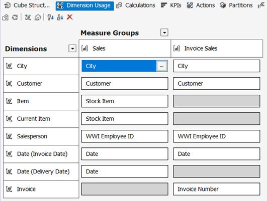
Figure 4.35 – Dimension Usage tab in the Cube Design window

Now that we have the dimensions set up, we can add more capabilities to our model.

Reviewing calculations and KPIs

The next two tabs are the focus of Chapter 5, Adding Measures and Calculations with MDX, where we'll dig into MDX and calculations. For now, you can skip these.

Creating an action

Actions are a great feature available in SSAS cubes. An action will allow you to drill through to details, open a report, or open a URL based on where you are in the data. It uses the data available to build out the action.

Note

Be aware that actions are not supported in all end user tools. For example, they are supported in Excel, but not in Power BI.

We will add a drillthrough action to our cube, as follows:

1. In the Actions tab of the Cube Design panel, right-click the Action Organizer pane and select New Drillthrough Action.
2. This will add the new action to the Action Organizer pane. You will see the properties for the action in the middle pane.
3. Rename the action Drill to Details.
4. Next, we need to select our drillthrough columns. In the Drillthrough Columns section, select the Item dimension table and choose all the fields.
5. On the next line, select Measures and choose the Quantity field.
6. On the next line, select Invoice Date and choose the Date field.
7. Process the cube. With that, your action should be in place. If you want to test it, you can use Excel to connect to the database and try it out. We will dig into using Excel in Chapter 9, Exploring and Visualizing Your Data with Excel.

Reviewing our partitions

On the Partitions tab, you will see the default partitions that have been created for our measure groups. Partitions physically separate the data in our measure groups into different buckets. These can be used to reduce processing time and effort for measure groups. While our cube does not require these since processing performance is fine in single partitions, let's walk through adding year partitions to the Sales measure group.

Our Sales measure group contains data from 2013 through 2016. We will create four partitions:

• 2013 and previous
• 2014
• 2015
• 2016 to Current

We will use the Partition Wizard to help us create our partitions. In production environments, you need to plan on creating new partitions as new data comes in. Some of those techniques will be covered later in this book. Let's get started:

1. Select Source in the Sales partition (line 1) and click the ellipsis (…) to open the Partition Source dialog box.
2. Change Binding Type to Query Binding.
3. Add [Sales].[Invoice Date Key] <= '12/31/2013' to the WHERE clause at the end. This will filter the current partition for dates from 2013 and earlier.
4. Rename the partition Sales 2013.
5. In the Properties pane, find EstimatedRows and set it to 61000. You can check the row count in SSMS by querying the source table with the same filter. When using partitions, this helps the aggregation wizard make better choices about aggregations.
6. Click New Partition… to launch the Partition Wizard window in order to create the next partition.
7. Click Next on the opening screen.
8. Select the Sales table on the Specify Source Information screen and click Next.
9. On the Restrict Rows screen, select Specify a query to restrict rows. This will open a query like the one we saw when we modified the first partition. Add [Sales].[Invoice Date Key] BETWEEN '1/1/2014' and '12/31/2014' to the WHERE clause. Check your work and click Next.
10. Leave the default values as is and click Next on the Processing and Storage Locations screen.
11. Rename the partition Sales 2014. Choose Design aggregations later and click Finish.
12. Follow the same process for the Sales 2015 partition.
13. Set EstimatedRows for the Sales 2014 partition to 70000.
14. Set EstimatedRows for the Sales 2015 partition to 75000.
15. For the Sales 2016 to Current partition, use [Sales].[Invoice Date Key] >= '1/1/2016' in the WHERE clause. Set EstimatedRows for this partition to 35000.

When you are done, your Partitions tab should have the following partitions for the Sales measure group:

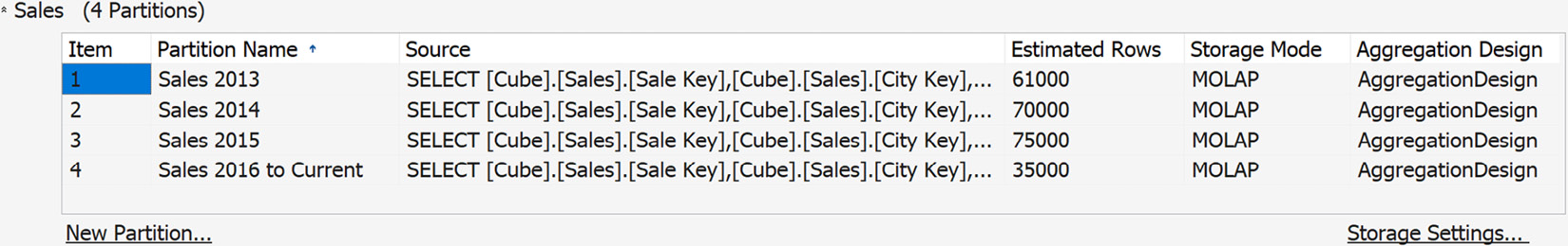
Figure 4.36 – Sales measure group partitions

We did not change the Storage Mode option. This option enables support for Relational Online Analytical Processing (ROLAP), which is used for direct relational querying from the cube. This is typically done to support real-time techniques so that we can view data changes as they occur. Multidimensional Online Analytical Processing (MOLAP) is typically the best option to choose for performance reasons. This is the default option and how multidimensional models are stored. Aggregations will be covered in the next section.

Process your model and resolve any errors. Next, we will add aggregations to our model.

Reviewing and creating aggregations

Aggregations are used to improve the query performance of your model. A balance has to be struck between too many aggregations, which can bloat the size of the model and ultimately hurt your processing and query performance, and too few aggregations, which keeps the cube smaller but makes performance an issue. When first creating a cube, the best plan is to let the Aggregation Design Wizard help you design them. Once you have deployed the model and there has been a lot of usage, you can use the Usage Based Optimization wizard to target aggregations to improve the user experience directly. For our model, we will use the Aggregation Design Wizard to create our initial aggregations.

Let's add aggregations to our Sales measure group:

1. Expand the Sales measure group on the Aggregations tab.
2. Right-click on Unassigned Aggregation Design and pick Design Aggregations to launch the wizard. Click Next on the opening screen.
3. You will see the partitions we created in the previous section. Select them all and click Next.
4. On the Review Aggregation Usage screen, you will see all the dimension attributes that can be targeted for aggregation. Default allows the wizard to decide on the amount of aggregation to use. The other settings should only be used if you have familiarity with the usage patterns and can provide guidance to the wizard. For our example, we will leave the defaults in place. Click Next.
5. The Specify Object Counts screen lets you enter estimates for the counts for all attribute and measure groups. Alternatively, you can click Count and the wizard will count them all. If you have any performance issues due to the size of the data, networking, or compute, you should enter the estimates yourself. Our dataset is small, so having the wizard count should not be an issue. Click Count. Once it's done this, you can expand the dimensions to see the counts. Click Next when you are done.
6. The next screen is Set Aggregations Options. The wizard will estimate and build an aggregation design based on the options selected. Storage will likely not be an issue for us. Performance Gain is a decent option for us to use here. I like to let it run and click Stop when it starts to slow down (meaning it is finding fewer options). You can choose any of these options. We are going to use the I click Stop option. Select that option, and then click Start to kick off the wizard. You can stop it whenever or let it run until it is done. The following screenshot shows where I stopped my wizard. Yours will likely look a bit different:
   

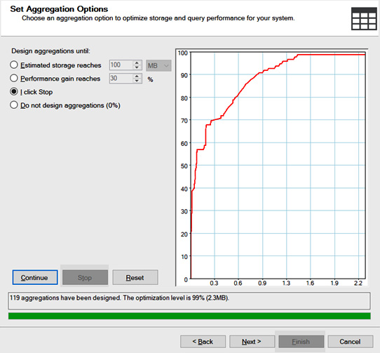
   Figure 4.37 – Aggregation Design Wizard completed with 99% optimization using 2.3 MB of storage

7. Click Next to move on to the final step.
8. Give the aggregation design a name, such as Initial Sales Aggregation, and choose the Save aggregations but do not process them option. Click Finish.

We can repeat this process for the Invoice Sales measure group. If you take a look at the Specify Object Count screen, you should notice that the counts are partially filled out based on the work we did with the Sales measure group. Now, process your project.

Reviewing and creating a perspective

Perspectives are like views in SQL Server databases. They allow you to create analytic views, which can make browsing the cube or creating reports easier. Let's create a simplified view of our Invoice Sales data:

1. Right-click in the empty space of the Perspectives tab. Choose New Perspective.
2. You will see that a new perspective has been added next to the Object Type column. Rename the perspective Invoicing.
3. Deselect the Sales measure group.
4. Deselect the City, Current Item, Item, Delivery Date, and Salesperson dimensions.
5. Only select Customer Hierarchy in the Customer dimension and Invoice Hierarchy in the Invoice dimension.
6. Only select the Invoice Total Including Tax and Invoice Count measures from the Invoice Sales measure group.
7. Save and process your model.

Reviewing translations

Translations allow you to supply a specific language for the names of dimensions, measures, and other viewable objects. You can also manage translations for dimension attributes on the Translations tab. You can do this for each dimension.

Browsing our cube

We have been building out a lot of functionality, and you have likely already used this to view your changes. We recommend processing the cube one more time to make sure all your changes are in place:

Figure 4.38 – Opening the cube browser

Here are some key things to be aware of in the browser:

1. This is the Change User button. You can choose which user experience you want to see. This is related to securing your cube data and can involve filtered objects and data.
2. This is the Reconnect button. Use this after processing your model so that you can see the latest changes.
3. This dropdown is how you toggle between MDX and DAX. In most cases, you will use MDX when working with multidimensional models.
4. This area is the filter area. You can drag a dimension here to limit the results of the query. Add a date filter here. Drag the Invoice Date dimension to this area. Leave Operator set to Equal. In Filter Expression, select CY2014. This will filter the results to invoice dates in calendar year 2014.
5. This is the metadata area. From here, you can drag measures, KPIs, and various dimension components, including the full dimension, hierarchies, and attributes, to the query area. You can also change the metadata view by selecting a different cube or perspective at the top. Click the button next to Wide World Importers at the top of the metadata and change the view to the Invoicing perspective.
6. This is the query area. You drop items from the metadata area here to build the query. You will see the results as you build. You need at least one measure and one dimension to see data here. Drag Bill To Customer from Customer Hierarchy, Invoice Count, and Invoice Total Including Tax to the query area. The results are filtered for CY2014. You should see the following output. Click the link in the query area to execute the query:

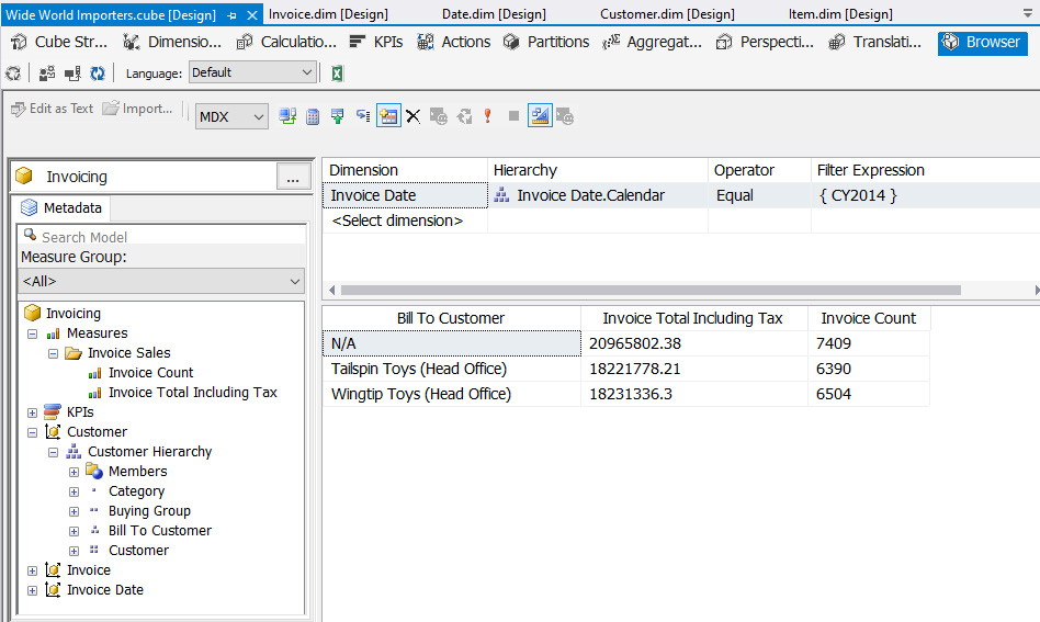
Figure 4.39 – Sample query using the cube browser

This concludes the build portion of the multidimensional model.

Summary

At this point, you have successfully created an Analysis Services multidimensional project. You have added dimensions and cubes to the project. You have also deployed your project as an Analysis Services database and processed that database so that you can load it with data. You now have a cube that supports basic analytics, which means you can browse the cube right now using tools such as Excel or Power BI. We wrapped up our build and deployment by browsing the data we deployed to the cube.

In the next chapter, we will continue to expand the cube by adding calculations and KPIs to it. We will also explore our data using SSMS and MDX.