Chapter 6: Preparing Your Data for Tabular Models

Tabular models are the newer analytics model structure implemented in SQL Server. The underlying analysis engine is columnar, not multidimensional, which means there are some different considerations for data preparation. The VertiPaq analysis engine was originally introduced in Excel and now supports Power BI datasets and Analysis Services tabular models. The technology behind VertiPaq uses a number of column-based algorithms to improve storage and performance. This technology allows Analysis Services to compress and structure the data for optimized performance. One other key design change is that tabular models match various relational data structures and are not reliant on a dimensional model for success.

In this chapter, we will look at the range of options, from minor preparation to star schema-based approaches. We will walk through prototyping tabular models with Excel Power Pivot capabilities. Because tabular models can be implemented without a lot of data prep at times, we will conclude the chapter by looking at some of the techniques needed to clean up projects that may have started out poorly. This chapter contains the information you need to build sustainable tabular models to drive business solutions for your organization.

In this chapter, we're going to cover the following main topics:

• Prepping data for tabular models
• Data optimization considerations
• Prototyping your model in Excel with Power Pivot

Technical requirements

In this chapter, we will be using the WideWorldImporters and WideWorldImportersDW databases from Chapter 1, Analysis Services in SQL Server 2019. You should connect to the database with SQL Server Management Studio (SSMS).

We will be using Excel to build the Power Pivot model prototype. For our examples, we will be using the Excel version that comes with Office 365 ProPlus. The other latest versions of Excel should allow you to participate in the hands-on examples as well.

Prepping data for tabular models

With multidimensional models, a star schema is required in the underlying data source. However, with tabular models, a star schema is not required. This means that data preparation is not as clear as it is with multidimensional models. In this section, we will explore some key considerations that are involved when preparing data for tabular models.

Contrasting self-service and managed deployments

Tabular model designs have their origins in self-service technologies such as Power BI and Excel. Why does this matter? Because well-designed dimensional models still perform better and are easier to develop solutions for. Self-service models often focus only on the immediate business need and not on lasting performance or growth. When the number of consumers of an analytics model is one or just a few, the impact is minimal. However, when scaling the models beyond a limited set of users, performance and usability become key considerations in design.

SQL Server Analysis Services tabular models are created in Visual Studio and managed at the server level. They are not self-service by nature. Technology development teams are responsible for maintaining, supporting, and enhancing these models. Those teams are also required to follow specific rules and processes to maintain the quality and functionality of the models.

A normal process in the industry is that when self-service models are difficult for the business to manage, they call on their internal technology teams to take them over. The problem with this scenario is that service-level agreements (SLAs), compliance requirements, and the overall need for security get in the way of business expectations. While this is not the focus of this book, you need to consider how to qualify tabular models as a different management process from self-service models.

Let's wrap this section up with a few contrasting points on the differences between self-service and managed deployments in the context of tabular model implementations in a business:

• Analysis Services tabular models support larger models than self-service tools. They are built on a server and can scale to the size of the memory in the server, which often exceeds the capabilities of the self-service environments.
• Self-service tools allow quicker changes due to the lack of controls and processes used when working with tabular models. This can be both good and bad. Self-service models can adapt quickly but are susceptible to bad data and processes that can lead to bad decisions being made. Tabular models take more time but are built around controls and processes to help achieve better data quality.
• Analysis Services tabular models are created with Visual Studio, a developer tool. Power BI and Excel are end user tools, which makes them easier to use and more approachable for designers of all levels. One key difference here is that Visual Studio projects have good source control and standard deployment options with versions that can be easily implemented by developers. This allows clear change tracking, which is not as easy to accomplish with self-service tools.

As you can see, the contrasts really come down to industry and corporate controls that have been traditionally managed by IT teams and model sizes. When these requirements become important, tabular models are required to support the business.

The impact of Power BI

Microsoft's Power BI product continues to change and fill gaps in enterprise implementations. Microsoft continues to invest in Power BI Premium, which has wider support for datasets and other additional capabilities. Power BI still has limitations in source control and other typical IT processes. Until the gap is closed, Analysis Services tabular models will continue to fill those needs for businesses with larger datasets and specific management controls for data and design.

Using a star schema data warehouse

The work that is required to create and maintain a star schema or dimensional data warehouse built on Kimball practices was described in detail in Chapter 3, Preparing Your Data for Dimensional Models. The principals behind a dimensional model make any analytics solution work well. A dimensional model is organized to support reporting and analysis with a focus on conformed dimensions and established measures.

A tabular model based on a dimensional data warehouse is one of the simplest implementations to do. In our case, we can use the star schemas we created in Chapter 3, Preparing Your Data for Dimensional Models, as shown in Figure 6.1. We created views to support two measure groups in the multidimensional model:

1. Sales: This has the detail-level sales for Wide World Importers. This star schema includes item-level sales:
   

   Figure 6.1 – Sales star schema views for Wide World Importers

2. Invoice Sales: This measure view has the data aggregated to the invoice. This pattern is very helpful in tabular models as it allows them to optimize for aggregations:

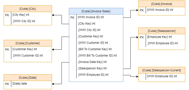
Figure 6.2 – Invoice sales star schema views for Wide World Importers

This is a case where the work is completed in the data warehouse and no additional preparations are required to support using this same schema with a tabular model. We will also look at some options that will support role-playing dimension design.

Role-playing dimensions in tabular models

Unlike multidimensional models, role-playing dimensions are not natively supported in the tabular model. In our case, we have role-playing relationships created with the Date dimension. The invoice and delivery dates are mapped to the same dimension.

Using non-star schema databases

When a tabular model is created on a database that has not been modeled with a star schema, you have a couple of options. The first option is obvious. Use the existing data structure as is and pull the data directly into the model. Using the tabular model features, you can rename columns to make them more user friendly. You can also add measures and columns to build out the model.

The other consideration is shaping the data before landing it in the model. This can be done using the Power Query feature in tabular model design. For example, Power Query can remove unused columns and add columns during the load process, as shown in the following screenshot:

Figure 6.3 – Power Query example

Power Query can be used to filter data, add and remove columns, and format data for use in the tabular model. This allows us to bypass loading star schema databases in simpler operations. The key consideration here is that the data will be transformed during the refresh process and the operations may not be as efficient as we see in modern extraction, transformation, and load (ETL) tools such as SQL Server Integration Services (SSIS).

Using nontraditional sources

One of the key characteristics in a data warehouse is that the source of the data for the analytics and reporting systems is one single source. Report and dashboard designers know that the data they are looking for is organized and managed by the data warehouse team and should be able to be trusted. However, today's analytics needs do not always make it to the data warehouse. Marketing teams are a great example of a group whose needs change constantly. They use tools such as Google Analytics, Facebook, and even YouTube to collect data and build reports. Often, these systems are not included in the data warehouse, and adding them is complicated.

Power Query allows model designers to add these data sources to tabular models and shape the data to allow it to be mashed up with a data warehouse or other traditional data sources. While this may not be the best long-term solution, it allows the data warehouse and analytics teams to create solutions quickly to support the business. If the business team is using Power Query in Power BI to collect this data initially, that work can be used to provide guidance and code to add to the larger tabular model projects.

The other common use case for data outside of the data warehouse is as general-purpose data managed by a third party. We often see weather, traffic, and census data sourced from third parties, including governments. The cost of pulling that data into a warehouse via traditional means typically results in a low return on investment. With the Power Query capability in SQL Server 2019 Analysis Services, businesses can add that data with minimal impact. More importantly, the third party will be responsible for quality and freshness, not the business teams.

Data optimization considerations

Another consideration when preparing your data for tabular models is the data refresh options available. Typically, data is imported into your tabular model similar to the process we used with multidimensional models. Imported data is loaded into memory and optimized by the VertiPaq engine. This involves a high level of compression, including columnar data storage techniques. The functions of compression and memory combine to create an optimized model with performance. Here are some key considerations when using data refresh:

• Refresh frequency: The data is only as fresh as the last import. If the data source has been updated recently, the data may be out of sync. This is less of an issue when you are loading data from a data warehouse. The data warehouse is typically loaded in batches as well. If you match your refreshes to the batch loads, your data will be consistent with the data warehouse. If you have chosen to use the transactional database for the source, that database is written frequently too. Thus, your data will only be as fresh as the latest import.
• Refresh time: Because the refresh process is importing the data into the model, you must consider the time for doing that operation. If you have used Power Query to shape a significant amount of your data, that will add to the refresh time because all data will need to be reshaped each time. You can partition the data to reduce the processing time in tabular models.
• Query performance: The import option has the best query performance. The data that is loaded into memory has been optimized for queries. Your users will notice the performance improvement in most cases. Typically, imported tabular models perform better than multidimensional models and DirectQuery tabular models.

The other data refresh option in tabular models is DirectQuery. DirectQuery does not import data into SQL Server Analysis Services. It uses the data source's engine to execute the queries. In our example, a DirectQuery model built on the data warehouse would send SQL statements to the data warehouse to fulfill user requests. The user experience will look like the import method, but the data is returned directly from the data warehouse, and not from memory in Analysis Services. Here are some key considerations when working with DirectQuery:

• Real-time connection: The data being served to users via DirectQuery is "real time" from the data source. Changes in the source will immediately be reflected in the user experience. DirectQuery makes it possible to have operational dashboards in tabular models. The other consideration here is that the data is dependent on the performance of the underlying source, and the network connectivity between the tabular model and the data source.
• One data source: DirectQuery has limited data source support. The first limitation is that a tabular model using DirectQuery can only use one data source. You cannot mash up data in DirectQuery. Secondly, DirectQuery only supports a limited set of relational sources at this time, including SQL Server, Azure SQL Database, Oracle, and Teradata.
• Not limited by memory: DirectQuery tabular models are not limited in size compared to the memory in Analysis Services. Because the data is returned from the data source data system, all the data is available for analysis. However, there is a limit on the number of rows returned – one million – although this can be adjusted if required.

As you can see, tabular models have flexibility in their storage and query capabilities. We recommend that you always start with the import mode and only use DirectQuery when you have a specific use case that requires it.

Now that we have looked at the tabular model refresh options, let's look at using Excel to create a tabular model.

Prototyping your model in Excel with Power Pivot

One of the cool things about using tabular models is that you can prototype your model using Excel. In this section, we will walk through creating a PowerPivot model to demonstrate building a prototype that we will upload to SQL Server Analysis Services in Chapter 7, Building a Tabular Model in SSAS 2019. We will work with the Invoice Sales star schema illustrated in Figure 6.2 earlier in this chapter. Let's get started:

1. Open Excel and create a new workbook. Power Pivot is built in, so no additional installs or extensions are required.
2. Next, we need to open the Power Pivot window. Go to the Data tab in Excel and click the Go to the Power Pivot Window button on the ribbon as shown in the following screenshot:
   

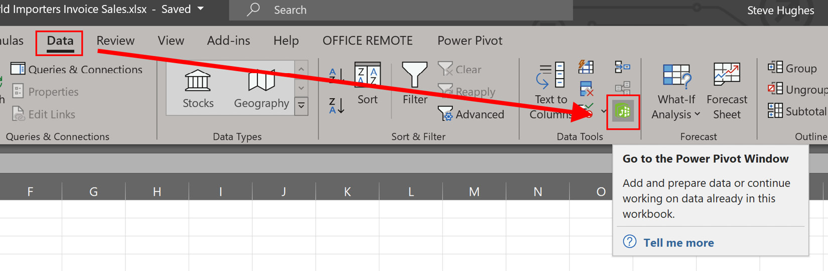
   Figure 6.4 – Opening Power Pivot in Excel

   If you have never opened Power Pivot before, you will be prompted to enable the Data Analysis features. You should now see a new window open with a ribbon as shown in the following screenshot:

   

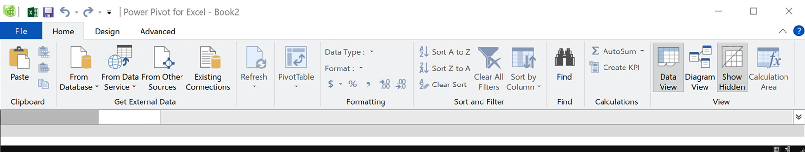
   Figure 6.5 – Power Pivot window

3. Connect to the WideWorldImportersDW database by choosing From Database and selecting From SQL Server. This will open the Table Import Wizard, as shown in the following screenshot:
   

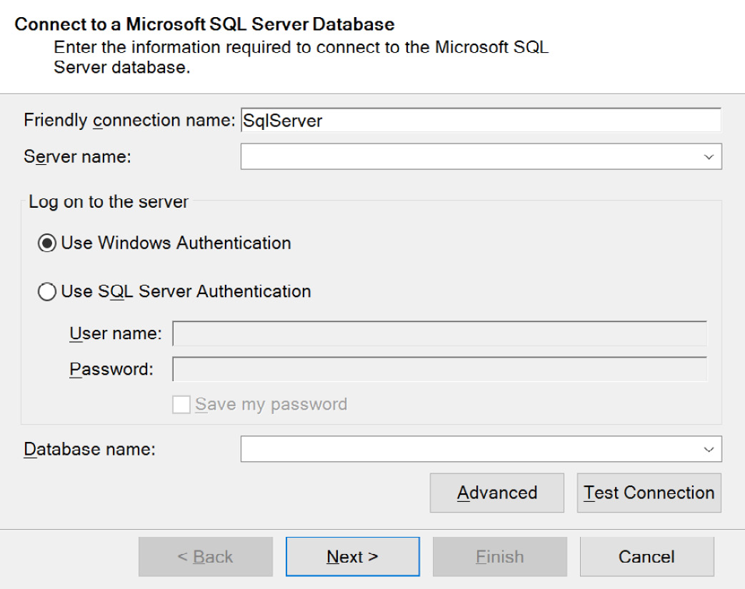
   Figure 6.6 – Table Import Wizard in Power Pivot

4. Fill in the connection information for your WideWorldImportersDW server and database and click Next >.
5. In the next screen, choose Select from a list of tables and views to choose the data to import and click Next >.
6. Select the following views from the Cube schema in the Select Tables and Views dialog: City, Customer, Date, Invoice, Invoice Sales, and Salesperson. You can leave the Friendly Name column. You should note that this dialog will try to create friendly names by recognizing syntax such as case and underscores. When you have selected those views, click Finish to load the data into Power Pivot as shown in the following screenshot:
   

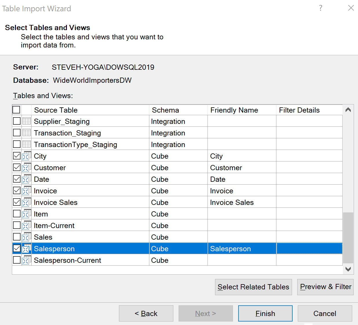
   Figure 6.7 – Select the views from the cube schema

   Be wary of the amount of data in your sources

   This process will try to load all the data from the selected tables into Power Pivot, which will consume memory on the device you are using. You should always use caution when using this feature or your device may run out of memory if the dataset you select is too large.

7. When the process is completed, you should see a dialog with the row counts for the views that were imported. You can close the window if it looks similar to mine, as shown in the following screenshot:
   

   Figure 6.8 – Pivot table successfully loaded

8. Review the imported data. You should see six tabs, one for each view we created. Before we move to the next step, let's get a short tour of Power Pivot using the following screenshot as reference. In the center of the screen is the data that has been imported into Power Pivot. To the right of the data you can see the option to add another column, which we will do shortly. Below the data is the Calculation Area, which is used to create measures:
   

   Figure 6.9 – Power Pivot data view

9. We also need to create relationships, as there were no foreign keys. You can create relationships using the Create Relationships button on the Design tab. However, it can be helpful to use Diagram View to create and view the relationships visually. Click Diagram View in the ribbon to change the view.
10. To create relationships, drag each dimension key onto the Invoice Sales fact table to the matching key. For example, drag the Date field from the Date table to Invoice Date Key in the Invoice Sales table. We rearranged the tables to look like a star schema. The following screenshot shows the rest of the relationships laid out:
    

    Figure 6.10 – Power Pivot relationships

    The following table describes the relationships in detail:

    

    Figure 6.11 – Power Pivot relationships defined

11. To add a couple of calculations to support our model, let's go back to the Data View. Now, click on the Invoice Sales tab. We will be adding two measures. The first will sum Invoice Total Including Tax and the other will calculate the average of Invoice Total Including Tax.
12. To create the sum, click any cell in the calculation area. We typically choose a cell near the column we are working with. Type in the following formula: Invoice Total:=sum('Invoice Sales'[Invoice Total Including Tax]).
13. Add another calculation below Invoice Total. It will be Invoice Average. Use the following code for this: Invoice Average:=AVERAGE('Invoice Sales'[Invoice Total Including Tax]).
14. Go ahead and set the format for both measures to currency ($ on the ribbon).
15. Go to the City tab. Let's add a calculated column with City and State Province. Click on Add Column and then add this to the formula: =City[City] & ", " & City[State Province]. Rename the column City and State.
16. Let's give our model a test run. On the ribbon, click PivotTable. This will create a PivotTable in Excel, connected to our model. In the new PivotTable, add our new measures from the Invoice Sales section to the Values section. Then add our new column, City and State, to Rows. Your PivotTable should look similar to the following screenshot:

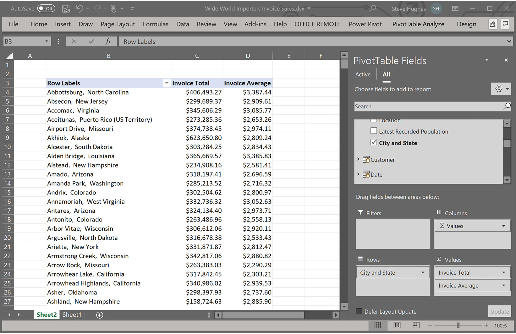
Figure 6.12 – PivotTable using our Power Pivot model

We will use the model in Chapter 7, Building a Tabular Model in SSAS 2019, to illustrate how to deploy this to Analysis Services. Using Power Pivot with Excel allows developers to build models locally and work with a rapid development and test cycle. When the model meets the needs of the business, they can easily promote the model to Analysis Services in most cases.

What about using Power BI to pivot?

Power BI can serve a similar purpose. It allows developers to rapidly build solutions and prototype in a similar and often easier way than Power Pivot in Excel. However, there is no automated way to promote the Power BI dataset to SQL Server Analysis Services right now. Power BI also has a more significant focus on the visualizations, whereas Power Pivot is focused on model creation.

Before we wrap up the chapter, save your Excel workbook with Power Pivot so we can use it for our later exercises in the coming chapters.

Summary

As you can see, data preparation is not as important for tabular models. In short, tabular models can be built quickly on less-than-great data structures. However, if you want to build models for a longer duration, it is best to build out a tried and true dimensional model. Once you have determined the foundation to build on, you can use that information to determine how you want to work with data – either via refresh or DirectQuery.

We also covered how to use Excel and Power Pivot to design and prototype an analytic model that can be imported into Analysis Services. Using Power Pivot is a great way to learn how to work with tabular model design, using Power Query to load and manipulate the data.

In the next chapter, we will build tabular models from the ground up in Visual Studio. We will also use the Power Pivot model we created in this chapter to create a new tabular model. Let's create some tabular models!