The Main Markets in Football

In American football, the three main markets have long been the spread, the total, and the moneyline. The spread, which is the most popular market, is pretty easy to understand: it is a point value meant to split outcomes in half over a large sample of games. Let’s consider an example. The Washington Commanders are—in a theoretical world where they can play an infinite number of games under the same conditions against the New York Giants—an average of four points better on the field. Oddsmakers would therefore make the spread between the Commanders and the Giants four points. With this example, five outcomes can occur for betting:

• A person bets for the Commanders to win. The Commanders win by five or more points, and the person wins their bet.

• A person bets for the Commanders to win. The Commanders lose outright or do not win by five or more points, and the person loses their bet.

• A person bets for the Giants to win. The Giants either win in the game outright or lose by three or fewer points, and the person wins their bet.

• A person bets for the Giants to win. The Giants lose outright, and the person loses their bet.

• A person bets for either team to win and the game lands on (the final score is) a four-point differential in favor of the Commanders. This game would be deemed a push, with the bettor getting their money back.

It’s expected that a point-spread bettor without an advantage over the sportsbook would win about 50% of their bets. This 50% comes from the understanding of probability, where the spread (theoretically) captures all information about the system. For example, betting on a coin being heads will be correct half the time and incorrect half the time over a long period. For the sportsbook to earn money off this player, it charges a vigorish, or vig, on each bet. For point-spread bets, this is typically 10 cents on the dollar.

Hence, if you wanted to win $100 betting Washington (–4), you would lay $110 to win $100. Such a bet requires a 52.38% success rate (computed by taking 110 / (110 + 100)) on nonpushed bets over the long haul to break even. Hence, to win at point-spread betting, you need roughly a 2.5-point edge (52.38%–50% is roughly 2.5%) over the sportsbook, which given the fact that over 99% of sports bettors lose money, is a lot harder than it sounds.

To bet a total, you simply bet on whether the sum of the two teams’ points goes over or under a specified amount. For example, say the Commanders and Giants have a market total of 43.5 points (–110); to bet under, you’d have to lay $110 to win $100 and hope that the sum of the Commanders’ and Giants’ points was 43 or less. Forty-four or more points would result in a loss of your initial $110 stake. No pushes are possible when the spread or total has a 0.5 tacked onto it. Some bettors specialize in totals, both full-game totals and totals that are applicable for only certain segments of the game (such as first half or first quarter).

The last of the traditional bets in American football is the moneyline bet. Essentially, you’re betting on a team to win the game straight up. Since a game is rarely a true 50-50 (pick’em) proposition, to bet a moneyline, you either have to lay a lot of money to win a little money (when a team is a favorite), or you get to bet a little money to win a lot of money (when a team is an underdog). For example, if the Commanders are considered 60% likely to win against the Giants, the Commanders would have a moneyline price (using North American odds, other countries use decimal odds) of –150; the bettor needs to lay $150 to win $100. The decimal odds for this bet are (100 + 150) / 150 = 1.67, which is the ratio of the total return to the investment. –150 is arrived at partially through convention—namely, the minus sign in front of the odds for a favorite, and through the computation of $100\times \frac{0.6}{(1-0.6)}=150$. The decimal odds here are (100 + 150) / 100 = 2.5.

The Giants would have a price of +150, meaning that a successful bet of $100 would pay out $150 in addition to the original bet. This is arrived at in the reciprocal way: $100\times \frac{1-0.4}{0.4}=150$, with the convention that the plus sign goes in front of the price for the underdog.

Application of Poisson Regression: Prop Markets

A model worth its salt in the three main football-betting markets using regression is beyond the scope of this book, as they require ratings for each team’s offense, defense, and special teams and require adjustments for things like weather and injuries. They are also the markets that attract the highest number of bettors and the most betting handle (or total amount of money placed by bettor), which makes them the most efficient betting markets in the US and among the most efficient betting markets in the world.

Since the overturning of PASPA, however, sportsbook operators have rushed to create alternatives for bettors who don’t want to swim in the deep seas of the spreads, totals, and moneylines of the football-betting markets. As a result, we see the proliferation of proposition (or prop) markets. Historically reserved for big events like the Super Bowl, now all NFL games and most college football games offer bettors the opportunity to bet on all kinds of events (or props): Who will score the first touchdown? How many interceptions will Patrick Mahomes have? How many receptions will Tyreek Hill have? Given the sheer volume of available wagers here, it’s much, much more difficult for the sportsbook to get each of these prices right, and hence a bigger opportunity for bettors to exist in these prop markets.

In this chapter, you’ll examine the touchdown pass market for NFL quarterbacks. Generally speaking, the quarterback starting a game will have a prop market of over/under 0.5 touchdown passes, over/under 1.5 touchdown passes, and for the very best quarterbacks, over/under 2.5 touchdown passes. The number of touchdown passes is called the index in this case. Since the number of touchdown passes a quarterback throws in a game is so discrete, the most important aspect of the prop offering is the price on over and under, which is how the markets create a continuum of offerings in response to bettors’ opinions.

Thus, for the most popular index, over/under 1.5 touchdown passes, one player might have a price of –140 (lay $140 to win $100) on the over, while another player may have a price of +140 (bet $100 to win $140) on over the same number of touchdown passes. The former is a favorite to go over 1.5 touchdown passes, while the latter is an underdog to do so. The way these are determined, and whether you should bet them, is determined largely by analytics.

The Poisson Distribution

To create or bet a proposition bet or participate in any betting market, you have to be able to estimate the likelihood, or probability, of events happening. In the canonical example in this chapter, this is the number of touchdown passes thrown by a particular quarterback in a given game.

The simplest way to try to specify these probabilities is to empirically look at the frequencies of each outcome: zero touchdown passes, one touchdown pass, two touchdown passes, and so on. Let’s look at NFL quarterbacks with at least 10 passing plays in a given week from 2016 to 2022 to see the frequencies of various touchdown-pass outcomes. We use the 10 passing plays threshold as a proxy for being the team’s starter, which isn’t perfect, but will do for now. Generally speaking, passing touchdown props are offered only for the starters in a given game. You will also use the same filter as in Chapter 5 to remove nonpassing plays. First, load the data in Python:

## Python
import pandas as pd
import numpy as np
import nfl_data_py as nfl
import statsmodels.formula.api as smf
import statsmodels.api as sm
import matplotlib.pyplot as plt
import seaborn as sns
from scipy.stats import poisson

seasons = range(2016, 2022 + 1)
pbp_py =
    nfl.import_pbp_data(seasons)

pbp_py_pass = 
  pbp_py.
    query('passer_id.notnull()')
    .reset_index()

Or load the data in R:

## R
library(nflfastR)
library(tidyverse)

pbp_r <-
    load_pbp(2016:2022)

pbp_r_pass <-
  pbp_r |>
  filter(!is.na(passer_id))

Then replace NULL or NA values with 0 for pass_touchdown. Python also requires plays without a passer_id and passer to be set to none so that the data will be summarized correctly.

Next, aggregate by season, week, passer_id, and passer to calculate the number of passes per week and the number of touchdown passes per week. Then, filter to exclude players with fewer than 10 plays as a passer for each week. Next, calculate the number of touchdown passes per quarterback per week.

Lastly, save the total_line because you will use this later. This is just nflfastR’s name for the market for total points scored, which we discussed earlier in this chapter. We assume that games with different totals will have different opportunities for touchdown passes (e.g., higher totals will have more touchdown passes, on average). The total_line is the same throughout a game, so you need to use a function so that Python or R can aggregate a value for the game. A function like mean() or max() will give you the value for the game, and we used mean(). Use this code in Python:

## Python
pbp_py_pass
    .loc[pbp_py_pass.pass_touchdown.isnull(), "pass_touchdown"] = 0

pbp_py_pass
    .loc[pbp_py_pass.passer.isnull(), "passer"] = 'none'

pbp_py_pass
    .loc[pbp_py_pass.passer_id.isnull(), "passer_id"] = 'none'

pbp_py_pass_td_y = 
    pbp_py_pass
    .groupby(["season", "week", "passer_id", "passer"])
    .agg({"pass_touchdown": ["sum"],
          "total_line": ["count", "mean"]})

pbp_py_pass_td_y.columns =
    list(map("_".join, pbp_py_pass_td_y.columns))

pbp_py_pass_td_y.reset_index(inplace=True)

pbp_py_pass_td_y
    .rename(columns={
        "pass_touchdown_sum": "pass_td_y",
        "total_line_mean": "total_line",
        "total_line_count": "n_passes"
    },
    inplace=True
)

pbp_py_pass_td_y =
    pbp_py_pass_td_y
   .query("n_passes >= 10")

pbp_py_pass_td_y
    .groupby("pass_td_y")
    .agg({"n_passes": "count"})

Resulting in:

           n_passes
pass_td_y
0.0             902
1.0            1286
2.0            1050
3.0             506
4.0             186
5.0              31
6.0               4

Or use this code in R:

## R
pbp_r_pass_td_y <-
    pbp_r_pass |>
    mutate(
        pass_touchdown = ifelse(is.na(pass_touchdown), 0,
                                pass_touchdown)) |>
    group_by(season, week, passer_id, passer) |>
    summarize(
        n_passes = n(),
        pass_td_y = sum(pass_touchdown),
        total_line = mean(total_line)
    ) |>
    filter(n_passes >= 10)

pbp_r_pass_td_y |>
    group_by(pass_td_y) |>
    summarize(n = n())

Resulting in:

# A tibble: 7 × 2
  pass_td_y     n
      <dbl> <int>
1         0   902
2         1  1286
3         2  1050
4         3   506
5         4   186
6         5    31
7         6     4

Now you can see why the most popular index is 1.5, since the meat of the empirical distribution is centered at around one touchdown pass, with players with at least ten pass attempts more likely to throw two or more touchdown passes than they are to throw zero. The mean of the distribution is 1.48 touchdown passes, as you can see here in Python:

## Python
pbp_py_pass_td_y
    .describe()

Resulting in:

            season         week    pass_td_y     n_passes   total_line
count  3965.000000  3965.000000  3965.000000  3965.000000  3965.000000
mean   2019.048928     9.620177     1.469609    38.798487    45.770618
std       2.008968     5.391064     1.164085    10.620958     4.409124
min    2016.000000     1.000000     0.000000    10.000000    32.000000
25%    2017.000000     5.000000     1.000000    32.000000    42.500000
50%    2019.000000    10.000000     1.000000    39.000000    45.500000
75%    2021.000000    14.000000     2.000000    46.000000    48.500000
max    2022.000000    22.000000     6.000000    84.000000    63.500000

Or in R:

pbp_r_pass_td_y |>
    ungroup() |>
    select(-passer, -passer_id) |>
    summary()

Resulting in:

     season          week          n_passes      pass_td_y      total_line
 Min.   :2016   Min.   : 1.00   Min.   :10.0   Min.   :0.00   Min.   :32.00
 1st Qu.:2017   1st Qu.: 5.00   1st Qu.:32.0   1st Qu.:1.00   1st Qu.:42.50
 Median :2019   Median :10.00   Median :39.0   Median :1.00   Median :45.50
 Mean   :2019   Mean   : 9.62   Mean   :38.8   Mean   :1.47   Mean   :45.77
 3rd Qu.:2021   3rd Qu.:14.00   3rd Qu.:46.0   3rd Qu.:2.00   3rd Qu.:48.50
 Max.   :2022   Max.   :22.00   Max.   :84.0   Max.   :6.00   Max.   :63.50

Counts of values are a good place to start, but sometimes you’ll need something more. In general, relying solely on these counts to make inferences and predictions has numerous issues. The most important issue that arises is one of generalization. This is where probability distributions come in handy.

Touchdown passes aren’t the only prop market in which you’re going to want to make bets; things like interceptions, sacks, and other low-frequency markets may all have similar quantitative features, and it would benefit you to have a small set of tools in the toolbox from which to work. Furthermore, other markets like passing yards, for which there are tenfold discrete outcomes, can often have more potential outcomes than outcomes that have occurred in the history of a league and, very likely, the history of a player. A general framework is evidently necessary here.

This is where probability distributions come in handy. A probability distribution is a mathematical object that assigns to each possible outcome a value between 0 and 1, called a probability. For discrete outcomes, like touchdown passes in a game, this is pretty easy to understand, and while it might require a formula to compute for each outcome, you can generally get the answer to the question “what is the probability that X = 0?” For outcomes that are continuous, like heights, it’s a bit more of a chore and requires tools from calculus. We will stick with using discrete probability distributions in this book.

One of the most popular discrete probability distributions is the Poisson distribution. This distribution defines the probability of obtaining the integer (that is, the discrete value) $x$ (such as $x=0,1,2,3,...$) as the value $\frac{e^{\lambda }{\lambda }^x}{x!}$. In this equation, the Greek letter $\lambda$ (lambda) is the average value of the population, and ! is the factorial function. The Poisson distribution models the likelihood of a given number of events occurring in a fixed interval of time or space.

Critical assumptions of the Poisson distribution are as follows:

• The events occur with equal probability.

• The events are independent of the time since the last event.

These assumptions are not exactly satisfied in football, as a team that scores one touchdown in a game may or may not be likely to have “figured out” the defense on the other side of the field, but it’s at least a distribution to consider in modeling touchdown passes in a game by a quarterback.

To see if a Poisson is reasonable, let’s look at a bar graph of the frequencies and compare this with the Poisson distribution of the same mean, $\lambda$. Do this using this Python code to create Figure 6-1:

## Python
pass_td_y_mean_py =
    pbp_py_pass_td_y
    .pass_td_y
    .mean()

plot_pos_py =
    pd.DataFrame(
        {"x": range(0, 7),
        "expected": [poisson.pmf(x, pass_td_y_mean_py) for x in range(0, 7)]
        }
    )

sns.histplot(pbp_py_pass_td_y["pass_td_y"], stat="probability");
plt.plot(plot_pos_py.x, plot_pos_py.expected);
plt.show();

Figure 6-1. Histogram (vertical bars) of normalized observed touchdowns per game per quarterback with at least 10 games (plotted with seaborn)

For this histogram, the term normalized refers to all the bars summing to 1. The line shows the theoretical expected values from the Poisson distribution.

Or, use this R code to create Figure 6-2:

## R
pass_td_y_mean_r <-
    pbp_r_pass_td_y |>
    pull(pass_td_y) |>
    mean()

plot_pos_r <-
    tibble(x = seq(0, 7)) |>
    mutate(expected = dpois(
        x = x,
        lambda = pass_td_y_mean_r
    ))

ggplot() +
    geom_histogram(
        data = pbp_r_pass_td_y,
        aes(
            x = pass_td_y,
            y = after_stat(count / sum(count))
        ),
        binwidth = 0.5
    ) +
    geom_line(
        data = plot_pos_r, aes(x = x, y = expected),
        color = "red", linewidth = 1
    ) +
    theme_bw() +
    xlab("Touchdown passes per player per game for 2016 to 2022") +
    ylab("Probability")

Figure 6-2. Histogram (vertical bars) of normalized observed touchdowns per game per quarterback with at least 10 games (plotted with ggplot2)

For this histogram, the normalized means that all the bars sum to 1. The line shows the theoretical expected values from the Poisson distribution. The Poisson distribution seems to slightly overestimate the likelihood of one touchdown pass, and as such, slightly underestimate the likelihood of zero, two, or more touchdown passes in a game.

Although not large, such discrepancies can be the difference between winning and losing in sports betting, so if you want to wager on your opinions, some adjustments need to be made. Alternatively, you could use a different distribution entirely (such as a negative binomial distribution or quasi-Poisson that accounts for over dispersion). But for the sake of this book, we’re going to assume that a Poisson distribution is sufficient to handicap touchdown pass probabilities in this chapter.

Individual Player Markets and Modeling

Each quarterback, and the player’s opponent, varies in quality, and hence each player will have a different market each game regarding touchdown passes. For example, in Super Bowl LVII between the Kansas City Chiefs and Philadelphia Eagles, Patrick Mahomes had a touch-down pass prop of 2.5 touchdown passes (per DraftKings Sportsbook), with the over priced at +150 (bet $100 to win $150) and the under priced at –185 (bet $185 to win $100).

As we’ve discussed, these prices reflect probabilities that you are betting against. In the case of the over, since the price is > 0, the formula for computing the break-even probability is 100 / (100 + 150) = 0.4. In other words, to bet the over, you have to be confident that Mahomes has better than a 40% chance to throw three or more touchdown passes against the Eagles defense, which ranked number one in the NFL during the 2022 season.

For the under, the break-even probability is 185 / (100 + 185) = 0.649, and hence you have to be more than 64.9% confident that Mahomes will throw for two or fewer touchdowns to make a bet on the under. Notice that these probabilities add to 104.9%, with the 4.9% representing the house edge, or hold, which is created by the book charging the vig discussed previously.

To specify these probabilities for Mahomes, you could simply go through the history of games Mahomes has played and look at the proportion of games with two or fewer touchdowns and three or more touchdowns to compare. This is faulty for a few reasons, the first of which is that it doesn’t consider exogenous factors like opponent strength, weather, changes to supporting cast, or similar factors. It also doesn’t factor changes to league-wide environments, like what happened during COVID-19, where the lack of crowd noise significantly helped offenses.

Now, you can incorporate this into a model in manifold ways, and anyone who is betting for real should consider as many factors as is reasonable. Here, you will use the aforementioned total for the game—the number of points expected by the betting markets to be scored. This factors in defensive strength, pace, and weather together as one number. In addition to this number, you will use as a feature the mean number of touchdown passes by the quarterback of interest over the previous two seasons.

## Python
for season_idx in range(2017, 2022 + 1):
    print(season_idx)
    for week_idx in range(1, 22 + 1):
        print(week_idx)

This is what you’re going to call x in your training of the model. With Python, use this code:

## Python
# pass_ty_d greater than or equal to 10 per week
pbp_py_pass_td_y_geq10 =
    pbp_py_pass_td_y.query("n_passes >= 10")

# take the average touchdown passes for each QB for the previous season
# and current season up to the current game
x_py = pd.DataFrame()
for season_idx in range(2017, 2022 + 1):
    for week_idx in range(1, 22 + 1):
        week_calc_py = (
            pbp_py_pass_td_y_geq10
                .query("(season == " +
                       str(season_idx - 1) +
                       ") |" +
                       "(season == " +
                       str(season_idx) +
                       "&" +
                       "week < " +
                       str(week_idx) +
                       ")")
            .groupby(["passer_id", "passer"])
            .agg({"pass_td_y": ["count", "mean"]})
        )
        week_calc_py.columns =
            list(map("_".join, week_calc_py.columns))
        week_calc_py.reset_index(inplace=True)
        week_calc_py
            .rename(columns={
                "pass_td_y_count": "n_games",
                "pass_td_y_mean": "pass_td_rate"},
            inplace=True)
        week_calc_py["season"] = season_idx
        week_calc_py["week"] = week_idx
        x_py = pd.concat([x_py, week_calc_py])

Or with R, use this code:

## R
# pass_ty_d greater than or equal to 10 per week
pbp_r_pass_td_y_geq10 <-
    pbp_r_pass_td_y |>
    filter(n_passes >= 10)

# take the average touchdown passes for each QB for the previous season
# and current season up to the current game
x_r <- tibble()

for (season_idx in seq(2017, 2022)) {
    for (week_idx in seq(1, 22)) {
        week_calc_r <-
            pbp_r_pass_td_y_geq10 |>
            filter((season == (season_idx - 1)) |
                (season == season_idx & week < week_idx)) |>
            group_by(passer_id, passer) |>
            summarize(
                n_games = n(),
                pass_td_rate = mean(pass_td_y),
                .groups = "keep"
            ) |>
            mutate(season = season_idx, week = week_idx)

        x_r <- bind_rows(x_r, week_calc_r)
    }
}

Notice here for every player going into each week, you have their average number of touchdown passes.

Let’s look at Patrick Mahomes going into Super Bowl LVII in Python:

## Python
x_py.query('passer == "P.Mahomes"').tail()

Resulting in:

     passer_id     passer  n_games  pass_td_rate  season  week
39  00-0033873  P.Mahomes       36      2.444444    2022    18
40  00-0033873  P.Mahomes       37      2.405405    2022    19
40  00-0033873  P.Mahomes       37      2.405405    2022    20
40  00-0033873  P.Mahomes       38      2.394737    2022    21
40  00-0033873  P.Mahomes       39      2.384615    2022    22

Or, let’s look in R:

## R
x_r |>
    filter(passer == "P.Mahomes") |>
    tail()

Resulting in:

# A tibble: 6 × 6
  passer_id  passer    n_games pass_td_rate season  week
  <chr>      <chr>       <int>        <dbl>  <int> <int>
1 00-0033873 P.Mahomes      35         2.43   2022    17
2 00-0033873 P.Mahomes      36         2.44   2022    18
3 00-0033873 P.Mahomes      37         2.41   2022    19
4 00-0033873 P.Mahomes      37         2.41   2022    20
5 00-0033873 P.Mahomes      38         2.39   2022    21
6 00-0033873 P.Mahomes      39         2.38   2022    22

Looks like the books set a decent number. Mahomes’s average prior to that game using data from 2021 and 2022 up to week 22 was 2.38 touchdown passes per game. You now have to create your response variable, which is simply the dataframe pbp_pass_td_y_geq10 created with the previous code along with the added game total. In Python, use a merge() function:

## Python
pbp_py_pass_td_y_geq10 =
    pbp_py_pass_td_y_geq10.query("season != 2016")
    .merge(x_py,
           on=["season", "week", "passer_id", "passer"],
           how="inner")

In R, use an inner_join() function (Appendix C provides more details on joins):

### R
pbp_r_pass_td_y_geq10 <-
    pbp_r_pass_td_y_geq10 |>
    inner_join(x_r,
        by = c(
            "season", "week",
            "passer_id", "passer"
        )
    )

You’ve now merged the datasets together to get your training dataset for the model. Before you model that data, quickly peek at it by using ggplot2 in R. First, plot passing touchdowns in each game for each passer by using a line (using the passer_id column rather than passer). In the plot, facet by season and add a meaningful caption. Save this as _weekly_passing_id_r_plot_ and look at Figure 6-3:

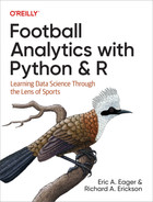
## R
weekly_passing_id_r_plot <-
    pbp_r_pass_td_y_geq10 |>
    ggplot(aes(x = week, y = pass_td_y, group = passer_id)) +
    geom_line(alpha = 0.25) +
    facet_wrap(vars(season), nrow = 3) +
    theme_bw() +
    theme(strip.background = element_blank()) +
    ylab("Total passing touchdowns") +
    xlab("Week of season")
weekly_passing_id_r_plot

Figure 6-3. Weekly passing touchdowns throughout the 2017 to 2022 seasons. Each line corresponds to an individual passer.

Figure 6-3 shows the variability in the passing touchdowns per game. The values seem to be constant through time, and no trends appear to emerge. Add a Poisson regression trend line to the plot to create Figure 6-4:

## R
weekly_passing_id_r_plot +
    geom_smooth(method = 'glm', method.args = list("family" = "poisson"),
                se=FALSE,
                linewidth = 0.5, color = 'blue',
                alpha = 0.25)

At first glance, no trends emerge in Figure 6-4. Players generally have a stable expected total passing touchdowns per game over the course of the seasons, with substantial variation week to week. Next, you’ll investigate this data by using a model.

Figure 6-4. Weekly passing touchdowns throughout the 2017 to 2022 seasons. Each line corresponds to an individual passer. The trendline is from a Poisson regression.

Since you are assuming a Poisson distribution for the number of touchdown passes thrown in a game by a player, you use a Poisson regression as your model. The code to fit a Poisson regression is similar to a logistic regression from Chapter 5. However, the family is now Poisson rather than binomial. Poisson is required to do a Poisson regression. In Python, use this code to fit the model, save the outputs to the column in the data called exp_pass_td, and look at the summary:

## Python
pass_fit_py = 
    smf.glm(
        formula="pass_td_y ~ pass_td_rate + total_line",
        data=pbp_py_pass_td_y_geq10,
        family=sm.families.Poisson())
    .fit()

pbp_py_pass_td_y_geq10["exp_pass_td"] = 
    pass_fit_py
    .predict()

print(pass_fit_py.summary())

Resulting in:

                 Generalized Linear Model Regression Results
==============================================================================
Dep. Variable:              pass_td_y   No. Observations:                 3297
Model:                            GLM   Df Residuals:                     3294
Model Family:                 Poisson   Df Model:                            2
Link Function:                    Log   Scale:                          1.0000
Method:                          IRLS   Log-Likelihood:                -4873.8
Date:                Sun, 04 Jun 2023   Deviance:                       3395.2
Time:                        09:41:29   Pearson chi2:                 2.83e+03
No. Iterations:                     5   Pseudo R-squ. (CS):            0.07146
Covariance Type:            nonrobust
================================================================================
                   coef    std err          z      P>|z|      [0.025      0.975]
--------------------------------------------------------------------------------
Intercept       -0.9851      0.148     -6.641      0.000      -1.276      -0.694
pass_td_rate     0.3066      0.029     10.706      0.000       0.251       0.363
total_line       0.0196      0.003      5.660      0.000       0.013       0.026
================================================================================

Likewise, in R use the following code to fit the model, save the outputs to the column in the data called exp_pass_td (note that you need to use type = "response" to put the output on the data scale rather than the coefficient/model scale), and look at the summary:

## R
pass_fit_r <-
    glm(pass_td_y ~ pass_td_rate + total_line,
        data = pbp_r_pass_td_y_geq10,
        family = "poisson"
    )

pbp_r_pass_td_y_geq10 <-
    pbp_r_pass_td_y_geq10 |>
    ungroup() |>
    mutate(exp_pass_td = predict(pass_fit_r, type = "response"))

summary(pass_fit_r) |>
    print()

Resulting in:

Call:
glm(formula = pass_td_y ~ pass_td_rate + total_line, family = "poisson",
    data = pbp_r_pass_td_y_geq10)

Coefficients:
              Estimate Std. Error z value Pr(>|z|)
(Intercept)  -0.985076   0.148333  -6.641 3.12e-11 ***
pass_td_rate  0.306646   0.028643  10.706  < 2e-16 ***
total_line    0.019598   0.003463   5.660 1.52e-08 ***
---
Signif. codes:  0 '***' 0.001 '**' 0.01 '*' 0.05 '.' 0.1 ' ' 1

(Dispersion parameter for poisson family taken to be 1)

    Null deviance: 3639.6  on 3296  degrees of freedom
Residual deviance: 3395.2  on 3294  degrees of freedom
AIC: 9753.5

Number of Fisher Scoring iterations: 5

Look at the coefficients and let’s interpret them here. For the Poisson regression, coefficients are on an exponential scale (see the preceding warning on this topic for extra details). In Python, access the model’s parameters and then take the exponential by using the NumPy library (np.exp()):

## Python
np.exp(pass_fit_py.params)

Resulting in:

Intercept       0.373411
pass_td_rate    1.358860
total_line      1.019791
dtype: float64

In R, use the tidy() function to look at the coefficients:

## R
library(broom)
tidy(pass_fit_r, exponentiate = TRUE, conf.int = TRUE)

Resulting in:

# A tibble: 3 × 7
  term         estimate std.error statistic  p.value conf.low conf.high
  <chr>           <dbl>     <dbl>     <dbl>    <dbl>    <dbl>     <dbl>
1 (Intercept)     0.373   0.148       -6.64 3.12e-11    0.279     0.499
2 pass_td_rate    1.36    0.0286      10.7  9.55e-27    1.28      1.44
3 total_line      1.02    0.00346      5.66 1.52e- 8    1.01      1.03

First, look at the pass_td_rate coefficient. For this coefficient, multiply every additional touchdown pass in the player’s history by 1.36 to get the expected number of touchdown passes. Second, look at the total_line coefficient. For this coefficient, multiply the total line by 1.02. In this case, the total line is pretty efficient and is within 2% of the expected value (1 – 1.02 = –0.02). Both coefficients differ statistically from 0 on the (additive) model scale or differ statistically from 1 on the (multiplicative) data scale.

Now, look at Mahomes’s data from Super Bowl LVII, leaving out the actual result for now (as well as the passer_id to save space) in Python:

## Python
# specify filter criteria on own line for space
filter_by = 'passer == "P.Mahomes" & season == 2022 & week == 22'
# specify columns on own line for space
cols_look = [
    "season",
    "week",
    "passer",
    "total_line",
    "n_games",
    "pass_td_rate",
    "exp_pass_td",
]

pbp_py_pass_td_y_geq10.query(filter_by)[cols_look]

Resulting in:

      season  week     passer  total_line  n_games  pass_td_rate  exp_pass_td
3295    2022    22  P.Mahomes        51.0       39      2.384615     2.107833

Or look at the data in R:

## R
pbp_r_pass_td_y_geq10 |>
    filter(passer == "P.Mahomes",
           season == 2022, week == 22) |>
    select(-pass_td_y, -n_passes, -passer_id, - week, -season, -n_games)

Resulting in:

# A tibble: 1 × 4
  passer    total_line pass_td_rate exp_pass_td
  <chr>          <dbl>        <dbl>       <dbl>
1 P.Mahomes         51         2.38        2.11

Now, what are these numbers?

• n_games shows that there are a total of 39 games (21 from the 2022 season and 18 from the previous season) in the Mahomes sample that we are considering.

• pass_td_rate is the current average number of touchdown passes per game by Mahomes in the sample that we are considering.

• exp_pass_td is the expected number of touchdown passes from the model for Mahomes in the Super Bowl.

And what do the numbers mean? These numbers show that Mahomes is expected to go under his previous average, even though his game total of 51 is relatively high. Likely, part of the concept of expected touchdown passes results from the concept of regression toward the mean. When people are above average, statistical models expect them to decrease to be closer to average (and the converse is true as well: below average players are expected to increase to be closer to the average). Because Mahomes is the best quarterback in the game at this point, the model predicts he is more likely to have a decrease rather than an increase. See Chapter 3 for more discussion about regression toward the mean.

Now, the average number doesn’t really tell you that much. It’s under 2.5, but the betting market already makes under 2.5 the favorite outcome. The question you’re trying to ask is “It is too much or too little of a favorite?” To do this, you can use exp_pass_td as Mahomes’s $\lambda$ value and compute these probabilities explicitly by using the probability mass function and cumulative density function.

A probability mass function (PMF) gives you the probability of a discrete event occurring, assuming a statistical distribution. With our example, this is the probability of a passer completing a single number of touchdown passes per game, such as one touchdown pass or three touchdown passes. A cumulative density function (CDF) gives you the sum of the probability of multiple events occurring, assuming a statistical distribution. With our example, this would be the probability of completing X or fewer touchdown passes. For example, using X = 2, this would be the probability of completing zero, one, and two touchdown passes in a given week.

Python uses relatively straightforward names for PMFs and CDFs. Simply append the name to a distribution. In Python, use poisson.pmf() to give the probability of zero, one, or two touchdown passes being scored in a game by a quarterback. Use 1 - poisson.cdf() to calculate the probability of more than two touchdown passes being scored in a game by a quarterback:

## Python
pbp_py_pass_td_y_geq10["p_0_td"] = 
    poisson.pmf(k=0,
                mu=pbp_py_pass_td_y_geq10["exp_pass_td"])

pbp_py_pass_td_y_geq10["p_1_td"] = 
    poisson.pmf(k=1,
                mu=pbp_py_pass_td_y_geq10["exp_pass_td"])

pbp_py_pass_td_y_geq10["p_2_td"] = 
    poisson.pmf(k=2,
                mu=pbp_py_pass_td_y_geq10["exp_pass_td"])

pbp_py_pass_td_y_geq10["p_g2_td"] = 
    1 - poisson.cdf(k=2,
                    mu=pbp_py_pass_td_y_geq10["exp_pass_td"])

From Python, look at the outputs for Mahomes going into the “big game” (or the Super Bowl, for readers who aren’t familiar with football):

## Python
# specify filter criteria on own line for space
filter_by = 'passer == "P.Mahomes" & season == 2022 & week == 22'

# specify columns on own line for space
cols_look = [
    "passer",
    "total_line",
    "n_games",
    "pass_td_rate",
    "exp_pass_td",
    "p_0_td",
    "p_1_td",
    "p_2_td",
    "p_g2_td",
]

pbp_py_pass_td_y_geq10
    .query(filter_by)[cols_look]

Resulting in:

         passer  total_line  n_games  ...    p_1_td    p_2_td   p_g2_td
3295  P.Mahomes        51.0       39  ...  0.256104  0.269912  0.352483

[1 rows x 9 columns]

R uses more confusing names for statistical distributions. The dpois() function gives the PMF, and the d comes from density because continuous distributions (such as the normal distribution) have density rather than mass. The ppois() function gives the CDF. In R, use the dpois() function to give the probability of zero, one, or two touchdown passes being scored in a game by a quarterback. Use the ppois() function to calculate the probability of more than two touchdown passes being scored in a game by a quarterback:

## R
pbp_r_pass_td_y_geq10 <-
    pbp_r_pass_td_y_geq10 |>
    mutate(
        p_0_td = dpois(x = 0,
                       lambda = exp_pass_td),
        p_1_td = dpois(x = 1,
                       lambda = exp_pass_td),
        p_2_td = dpois(x = 2,
                       lambda = exp_pass_td),
        p_g2_td = ppois(q = 2,
                        lambda = exp_pass_td,
                        lower.tail = FALSE)
    )

Then look at the outputs for Mahomes going into the big game from R:

## R
pbp_r_pass_td_y_geq10 |>
    filter(passer == "P.Mahomes", season == 2022, week == 22) |>
    select(-pass_td_y, -n_games, -n_passes,
           -passer_id, -week, -season)

Resulting in:

# A tibble: 1 × 8
  passer    total_line pass_td_rate exp_pass_td p_0_td p_1_td p_2_td p_g2_td
  <chr>          <dbl>        <dbl>       <dbl>  <dbl>  <dbl>  <dbl>   <dbl>
1 P.Mahomes         51         2.38        2.11  0.122  0.256  0.270   0.352

OK, so you’ve estimated a probability of 35.2% that Mahomes would throw three or more touchdown passes, which is under the 40% you need to make a bet on the over.¹ The 64.8% that he throws two or fewer touchdown passes is slightly less than the 64.9% we need to place a bet on the under.

As an astute reader, you will notice that this is why most sports bettors don’t win in the long term. At least at DraftKings Sportsbook, the math tells you not to make a bet or to find a different sportsbook altogether! FanDuel, one of the other major sportsbooks in the US, had a different index, 1.5 touchdowns, and offered –205 on the over (67.2% breakeven) and +164 (37.9%) on the under, which again offered no value, as we made the likelihood of one or fewer touchdown passes 37.8%, and two or more at 62.2%, with the under again just slightly under the break-even probability for a bet.

Luckily for those involved, Mahomes went over both 1.5 and 2.5 touchdown passes en route to the MVP. So the moral of the story is generally, “In all but a few cases, don’t bet.”

Poisson Regression Coefficients

The coefficients from a GLM depend on the link function, similar to the logistic regression covered in “A Brief Primer on Odds Ratios”. By default in Python and R, the Poisson regression requires that you apply the exponential function to be on the same scale as the data. However, this changes the coefficients on the link scale from being additive (like linear regression coefficients) to being multiplicative (like logistic regression coefficients).

To demonstrate this property, we will first use a simulation to help you better understand Poisson regression. First, you’ll consider 10 draws (or samples) from a Poisson distribution with a mean of 1 and save this to be object x. Then look at the values for x by using print(), as well as the mean.

In Python, use this code to generate the random numbers:

## Python
from scipy.stats import poisson

x = poisson.rvs(mu=1, size=10)

Then print the numbers:

## Python
print(x)

Resulting in:

[1 1 1 2 1 1 1 4 1 1]

And print their mean:

## Python
print(x.mean())

Resulting in:

1.4

In R, use this code to generate the numbers:

## R
x <- rpois(n = 10, lambda = 1)

And then print the numbers:

## R
print(x)

Resulting in:

 [1] 2 0 6 1 1 1 3 0 1 1

And then look at their mean:

## R
print(mean(x))

Resulting in:

[1] 1.6

Next, fit a GLM with a global intercept and look at the coefficient on the model scale and the exponential scale. In Python, use this code:

# Python
import statsmodels.formula.api as smf
import statsmodels.api as sm
import numpy as np
import pandas as pd

# create dataframe for glm
df_py = pd.DataFrame({"x": x})

# fit GLM
glm_out_py = 
    smf.glm(formula="x ~ 1", data=df_py, family=sm.families.Poisson()).fit()

# Look at output on model scale
print(glm_out_py.params)

# Look at output on exponential scale

Resulting in:

Intercept    0.336472
dtype: float64

print(np.exp(glm_out_py.params))

Resulting in:

Intercept    1.4
dtype: float64

In R, use this code:

## R
library(broom)

# fit GLM
glm_out_r <-
    glm(x ~ 1, family = "poisson")

# Look at output on model scale
print(tidy(glm_out_r))

Resulting in:

# A tibble: 1 × 5
  term        estimate std.error statistic p.value
  <chr>          <dbl>     <dbl>     <dbl>   <dbl>
1 (Intercept)    0.470     0.250      1.88  0.0601

# Look at output on exponential scale
print(tidy(glm_out_r, exponentiate = TRUE))

Resulting in:

# A tibble: 1 × 5
  term        estimate std.error statistic p.value
  <chr>          <dbl>     <dbl>     <dbl>   <dbl>
1 (Intercept)     1.60     0.250      1.88  0.0601

Notice that the coefficient on the exponential scale (the second printed table, with exponentiate = TRUE) is the same as the mean of the simulated data. However, what if you have two coefficients, such as a slope and an intercept?

As a concrete example, consider the number of touchdowns per game for the Baltimore Ravens. During this season, the Ravens’ quarterback was unfortunately injured during game 13. Hence, you might reasonably expect the Ravens’ number of passes to decrease over the course of the season. A formal method to test this would be to ask the question “Does the average (or expected) number of touchdowns per game change through the season?” and then use a Poisson regression to statistically evaluate this.

To test this, first wrangle the data and then plot it to help you see what is going on with the data. You will also shift the week by subtracting 1. This allows week 1 to be the intercept of the model. You will also set the axis ticks and change the axis labels. In Python, use this code to create Figure 6-5:

## Python
# subset the data
bal_td_py = (
    pbp_py
    .query('posteam=="BAL" & season == 2022')
    .groupby(["game_id", "week"])
    .agg({"touchdown": ["sum"]})
)

# reformat the columns
bal_td_py.columns = list(map("_".join, bal_td_py.columns))
bal_td_py.reset_index(inplace=True)

# shift week so intercept 0 = week 1
bal_td_py["week"] = bal_td_py["week"] - 1

# create list of weeks for plot
weeks_plot = np.linspace(start=0, stop=18, num=10)
weeks_plot

# plot the data

Resulting in:

array([ 0.,  2.,  4.,  6.,  8., 10., 12., 14., 16., 18.])

ax = sns.regplot(data=bal_td_py, x="week", y="touchdown_sum");
ax.set_xticks(ticks = weeks_plot, labels = weeks_plot);
plt.xlabel("Week")
plt.ylabel("Touchdowns per game")

plt.show();

Figure 6-5. Ravens touchdowns per game during the 2022 season, plotted with seaborn. Notice the use of a linear regression trendline.

In R, use this code to create Figure 6-6:

## r
bal_td_r <-
    pbp_r |>
    filter(posteam == "BAL" & season == 2022) |>
    group_by(game_id, week) |>
    summarize(
        td_per_game =
            sum(touchdown, na.rm = TRUE),
        .groups = "drop"
    ) |>
    mutate(week = week - 1)

ggplot(bal_td_r, aes(x = week, y = td_per_game)) +
    geom_point() +
    theme_bw() +
    stat_smooth(
        method = "glm", formula = "y ~ x",
        method.args = list(family = "poisson")
    ) +
    xlab("Week") +
    ylab("Touchdowns per game") +
    scale_y_continuous(breaks = seq(0, 6)) +
    scale_x_continuous(breaks = seq(1, 20, by = 2))

Figure 6-6. Ravens touchdowns per game during the 2022 season, plotted with ggplot2. Notice the use of a Poisson regression trend line.

When comparing Figures 6-5 and 6-6, notice that ggplot2 allows you to use a Poisson regression for the trendline, whereas seaborn allows only a liner model. Both figures show that Baltimore, on average, has a decreasing number of touchdowns per game. Now, let’s build a model and look at the coefficients. Here’s the code in Python:

## Python
glm_bal_td_py = 
    smf.glm(formula="touchdown_sum ~ week",
            data=bal_td_py,
            family=sm.families.Poisson())
    .fit()

Then look at the coefficients on the link (or log) scale:

## Python
print(glm_bal_td_py.params)

Resulting in:

Intercept    1.253350
week        -0.063162
dtype: float64

And look at the exponential (or data) scale:

## Python
print(np.exp(glm_bal_td_py.params))

Resulting in:

Intercept    3.502055
week         0.938791
dtype: float64

Or use R to fit the model:

## R
glm_bal_td_r <-
    glm(td_per_game ~ week,
        data = bal_td_r,
        family = "poisson"
    )

Then look at the coefficient on the link (or log) scale:

## R
print(tidy(glm_bal_td_r))

Resulting in:

# A tibble: 2 × 5
  term        estimate std.error statistic    p.value
  <chr>          <dbl>     <dbl>     <dbl>      <dbl>
1 (Intercept)   1.25      0.267       4.70 0.00000260
2 week         -0.0632    0.0300     -2.10 0.0353

And look at the exponential (or data) scale:

## R
print(tidy(glm_bal_td_r, exponentiate = TRUE))

Resulting in:

# A tibble: 2 × 5
  term        estimate std.error statistic    p.value
  <chr>          <dbl>     <dbl>     <dbl>      <dbl>
1 (Intercept)    3.50     0.267       4.70 0.00000260
2 week           0.939    0.0300     -2.10 0.0353

Now, let’s look the meaning of the coefficients. First, examining the link-scale value of the intercept, 1.253, and the slope, -0.063, does not appear to provide much context. However, the slope term is also known as the risk ratio, or relative risk, for each week. After exponentiating the coefficients, you get an intercept value of 3.502 and a slope value of 0.939.

These numbers do have easy-to-understand values. The intercept is the number of expected passes during the first game (this is why we had you subtract 1 from week, so that week 1 would be 0 and the intercept), and its value is 3.502. Looking at Figures 6-5 and 6-6, this seems reasonable because week 0 was 3 and weeks 1 and 2 were 5.

Then, for the next week, the expected number of touchdowns would be $3.502\times 0.939=3.288$. For the following week, $3.502\times 0.{939}^2=3.088$. Hence, the equation to estimate the expected number of touchdowns for a given week during the 2022 season for the Baltimore Ravens would be $3.502\times 0.{939}^{\mathrm{week}}$ on the log scale. Or this could be rewritten as $e^{1.253+-0.063\times \mathrm{week}}$.

Although we had to cherry-pick this example to explain a Poisson regression, hopefully the example served its purpose and helps you see how to interpret Poisson regression terms.

Closing Thoughts on GLMs

This chapter and Chapter 5 have introduced you to GLMs and how the models can help you both understand and predict with data. In fact, the simple predictions done in these chapters would help you also understand the basics of simple machine learning methods. When working with GLMs, notice that both example models forced you to deal with the link function because the coefficients are estimated on a different scale compared to the data. Additionally, you saw two types of error families, the binomial in Chapter 5 and the Poisson in this chapter.

In the exercises in this chapter, we have you look at the quasi-Poisson to account for dispersion when there are either too many or too few 0s compared to what would be expected. We also have you look at the negative binomial as another alternative to Poisson for modeling count data. Two other common types of GLMs include the gamma regression and the lognormal regression. The gamma and lognormal are similar. The lognormal might be better for some data that is positive but has a right skew as pass data (the data has more or greater positive values on the right side of the distribution and has smaller or negative values on the left side of the distribution).

An alphabet soup of extensions exists for linear models and GLMS. Hierarchical, multilevel, or random-effect models allow for features such as repeated observations on the same individual or group to model uncertainty. Generalized additive models (GAMs) allow for curves, rather than straight lines, to be fit for models. Generalized additive mixed-effect models (GAMMs) merge GAMs and random-effect models. Likewise, tools such as model selection can help you determine which type of model to use.

Basically, linear models have many options because of their long history and use in statistics and scientific fields. We have a colleague who can, and would, talk about the assumptions of regressions for hours on end. Likewise, year-long graduate-level courses exist on the models we have covered over the course of a few chapters. However, even simply knowing the basics of regression models will greatly help you to up your football analytics game.

Data Science Tools Used in This Chapter

This chapter covered the following topics:

• Fitting a Poisson regression in Python and R by using glm()

• Understanding and reading the coefficients from a Poisson regression including relative risk

• Connecting to datasets by using merge() in Python or an inner_join() in R

• Reapplying data-wrangling tools you learned in previous chapters

• Learning about betting odds

Exercises

1. What happens in the model for touchdown passes if you don’t include the total for the game? Does it change any of the probabilities enough to recommend a bet for Patrick Mahomes’s touchdown passes in the Super Bowl?

2. Repeat the work in this chapter for interceptions thrown. Examine Mahomes’s interception prop in Super Bowl LVII, which was 0.5 interceptions, with the over priced at –120 and the under priced at –110.

3. What about Jalen Hurts, the other quarterback in Super Bowl LVII, whose touchdown prop was 1.5 (–115 to the over and –115 to the under) and interception prop was 0.5 (+105/–135)? Was there value in betting either of those markets?

4. Look through the nflfastR dataset for additional features to add to the models for both touchdowns and interceptions. Does pregame weather affect either total? Does the size of the point spread?

5. Repeat this chapter’s GLMS, but rather than using a Poisson distribution, use a quasi-Poisson that estimates dispersion parameters.

6. Repeat this chapter’s GLMS, but rather than using Poisson distribution, use a negative binomial.

Suggested Readings

The resources suggested in “Suggested Readings” on pages 76, 112, and 136 will help you understand generalized linear models such as Poisson regression more. One last regression book you may find helpful is: Applied Generalized Linear Models and Multilevel Models in R by Paul Roback and Julie Legler (CRC Press, 2021). This book provides an accessible introduction for people wanting to learn more about regression analysis and advanced tools such as GLMs.

To learn more about the application of probability to both betting and the broader world, check out the following resources:

• The Logic of Sports Betting by Ed Miller and Matthew Davidow (self-published, 2019) provides details about how betting works for those wanting more details.

• The Wisdom of the Crowds by James Surowiecki (Doubleday, 2004) describes how “the market” or collective guess of the crowds can predict outcomes.

• Sharp Sports Betting by Stanford Wong (Huntington Press, 2021) will help readers understand betting more and provides an introduction to the topic.

• Sharper: a Guide to Modern Sports Betting by True Pokerjo (self-published, 2016) talks about sports betting for those seeking insight.

• The Foundations of Statistics, 2nd revised edition, by Leonard J. Savage (Dover Press, 1972) is a classical statistical text on how to use statistics to make decisions. The first half of the book does a good job explaining statistics in real-world application. The second becomes theoretical for those seeking a mathematically rigorous foundation. (Richard skimmed and then skipped much of the second half.)

• The Good Judgment Project seeks to apply the “wisdom of the crowds” to predict real-world problems. Initially funded by the US Intelligence Community, this project’s website states that its “forecasts were so accurate that they even outperformed intelligence analysts with access to classified data.”