Chapter 5. Generalized Linear Models: Completion Percentage over Expected
In Chapters 3 and 4, you used both simple and multiple regression to adjust play-by-play data for the context of the play. In the case of ball carriers, you adjusted for the situation (such as down, distance, yards to go) to calibrate individual player statistics on the play level, and later the season level. This approach clearly can be applied to the passing game, and more specifically, quarterbacks. As discussed in Chapter 3, Minnesota quarterback Sam Bradford set the NFL record for seasonal completion percentage in 2016, completing a whopping 71.6% of his passes.
Bradford, however, was just a middle-of-the-pack quarterback in terms of efficiency—whether measured by yards per pass attempt, expected points per passing attempt, or touchdown passes. The Vikings won only 7 of his 15 starts that year. The reason Bradford’s completion percentage was so high was that he averaged just 6.6 yards for depth per target (37th in the NFL, per PFF). In general, passes that are thrown longer distances are completed at a lower rate.
To see this, you will create Figure 5-1 in Python or Figure 5-2 in R. First, load the data. Then, filter pass plays (play_type == "pass") with a passer (passer_id.notnull() in Python or !is.na(passer_id) in R), and a pass depth (air_yards.notnull() in Python or !is.na(air_yards) in R). In Python, use this code:
## Pythonimportpandasaspdimportnumpyasnpimportnfl_data_pyasnflimportstatsmodels.formula.apiassmfimportstatsmodels.apiassmimportmatplotlib.pyplotaspltimportseabornassnsseasons=range(2016,2022+1)pbp_py=nfl.import_pbp_data(seasons)pbp_py_pass=pbp_py.query('play_type == "pass" & passer_id.notnull() &'+'air_yards.notnull()').reset_index()
Or with R, use this code:
## Rlibrary(tidyverse)library(nflfastR)library(broom)pbp_r<-load_pbp(2016:2022)pbp_r_pass<-pbp_r|>filter(play_type=="pass"&!is.na(passer_id)&!is.na(air_yards))
Next, restrict air yards to be greater than 0 yards and less than or equal to 20 yards in order to ensure that you have a large enough sample size. Summarize the data to calculate the completion percentage, comp_pct. Then plot results to create Figure 5-1:
## Python# Change theme for chaptersns.set_theme(style="whitegrid",palette="colorblind")# Format and then plotpass_pct_py=pbp_py_pass.query('0 < air_yards <= 20').groupby('air_yards').agg({"complete_pass":["mean"]})pass_pct_py.columns=list(map('_'.join,pass_pct_py.columns))pass_pct_py.reset_index(inplace=True)pass_pct_py.rename(columns={'complete_pass_mean':'comp_pct'},inplace=True)sns.regplot(data=pass_pct_py,x='air_yards',y='comp_pct',line_kws={'color':'red'});plt.show();

Figure 5-1. Scatterplot with linear trendline for air yards and completion percentage, plotted with seaborn
Or use R to create Figure 5-2:
## Rpass_pct_r<-pbp_r_pass|>filter(0<air_yards&air_yards<=20)|>group_by(air_yards)|>summarize(comp_pct=mean(complete_pass),.groups='drop')pass_pct_r|>ggplot(aes(x=air_yards,y=comp_pct))+geom_point()+stat_smooth(method='lm')+theme_bw()+ylab("Percent completion")+xlab("Air yards")
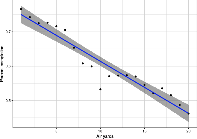
Figure 5-2. Scatterplot with linear trendline for air yards and completion percentage, plotted with ggplot2
Figures 5-1 and 5-2 clearly show a trend, as expected. Thus, any discussion of quarterback accuracy—as measured by completion percentage—needs to be accompanied by some adjustment for style of play.
Completion percentage over expected, referred to as CPOE in the football analytics world (and introduced in Chapter 1), is one of the adjusted metrics that has made its way into the mainstream. Ben Baldwin’s website, a great reference for open football data, displays CPOE as one of its main metrics in large part because CPOE together with EPA per passing play has shown to be the most predictive public metric for quarterback play from year to year. The NFL’s Next Generation Stats (NGS) group has its own version of CPOE, which includes tracking data-engineered features like receiver separation from nearest defender, prominently displayed on its website. ESPN uses the metric consistently in its broadcasts.
Measuring quarterback performance this way has some issues, which we will touch on at the end of the chapter, but CPOE is here to stay. We will start the process of walking you through its development by using generalized linear models.
Generalized Linear Models
Chapter 3 defined and described some key assumptions of simple linear regression. These assumptions included the following:
-
The predictor is linearly related to a single dependent variable, or feature.
-
One predictor variable (simple linear regression) or more predictor variables (multiple regression) describe the dependent variable.
Another key assumption of multiple regression is that the distribution of the residuals follows a normal, or bell-curve, distribution. Although almost all datasets violate this last assumption, usually the assumption works “well enough.” However, some data structures cause multiple regression to fail or produce nonsensical results. For example, completion percentage is a value bounded between 0 and 1 (bounded means the value cannot be smaller than 0 or larger than 1), as a pass is either incomplete (pass_complete = 0) or complete (pass_complete = 1). Hence a linear regression, which assumes no bounds on the response variable, is often inappropriate.
Likewise, other data commonly violates this assumption. For example, count data often has too many 0s to be normal and also cannot be negative (such as sacks per game). Likewise, binary data with two outcomes (such as win/lose or incomplete/complete pass) and discrete outcomes (such as passing location, which can be right, left, or middle) does not work with multiple regression as response data.
A class of regression models exists to model these types of outcomes: generalized linear models (GLMs). GLMs generalize, or extend, linear models to allow for response variables that are assumed to come from a non-normal distribution (such as binary responses or counts). The specific type of response distribution is called the family. One special type of GLM can be used to model binary data and is covered in this chapter. Chapter 6 covers how to use another type of GLM, the Poisson regression, with count data.
Other types of data can be analyzed by GLMs. For example, discrete outcomes can be analyzed using ordinal regression (also known as ordinal classification) but are beyond the scope of this book. Lastly, linear models (also known as linear regression and ordinary least squares) are a special type of a GLM—specifically, a GLM with a normal, or Gaussian, family.
To understand the basic theory behind how GLMs work, look at a completed pass that can be either 1 (completed) or 0 (incomplete). Because two outcomes are possible, this a binary response, and you can assume that a binomial distribution does a “good enough job” of describing the data. A normal distribution assumes two parameters: one for the center of the bell curve (the mean), and a second to describe the width of the bell curve (the standard deviation). In contrast, a binomial distribution requires only one parameter: a probability of success. With the pass example, this would be the probability of completing a pass. However, statistically modeling probability is hard because it is bounded by 0 and 1. So, a link function converts (or links) probability (a value ranging from 0 to 1) to a value ranging from
Building a GLM
To apply GLMs, and specifically a logistic regression, you will start with a simple example. Let’s begin by examining air_yards as our one feature for predicting completed passes. As suggested in Figures 5-1 and 5-2, longer passes are less likely to be completed. Now, you’ll use a model to quantify this relation.
With Python, use the glm() function from statsmodels.formula.api (imported as smf) as well as the binomial family from statsmodels.api (imported as sm) with the play-by-play data to fit a GLM and then look at the model fit’s summary:
## Pythoncomplete_ay_py=smf.glm(formula='complete_pass ~ air_yards',data=pbp_py_pass,family=sm.families.Binomial()).fit();complete_ay_py.summary()
Resulting in:
<class 'statsmodels.iolib.summary.Summary'>
"""
                 Generalized Linear Model Regression Results
==============================================================================
Dep. Variable:          complete_pass   No. Observations:               131606
Model:                            GLM   Df Residuals:                   131604
Model Family:                Binomial   Df Model:                            1
Link Function:                  Logit   Scale:                          1.0000
Method:                          IRLS   Log-Likelihood:                -81073.
Date:                Sun, 04 Jun 2023   Deviance:                   1.6215e+05
Time:                        09:37:33   Pearson chi2:                 1.32e+05
No. Iterations:                     5   Pseudo R-squ. (CS):            0.07013
Covariance Type:            nonrobust
==============================================================================
                 coef    std err          z      P>|z|      [0.025      0.975]
------------------------------------------------------------------------------
Intercept      1.0720      0.008    133.306      0.000       1.056       1.088
air_yards     -0.0573      0.001    -91.806      0.000      -0.059      -0.056
==============================================================================
"""
Likewise, with R, use the glm() function that is included with the core R packages, include a binomial family, and then look at the summary:
## Rcomplete_ay_r<-glm(complete_pass~air_yards,data=pbp_r_pass,family="binomial")summary(complete_ay_r)
Resulting in:
Call:
glm(formula = complete_pass ~ air_yards, family = "binomial",
    data = pbp_r_pass)

Coefficients:
              Estimate Std. Error z value Pr(>|z|)
(Intercept)  1.0719692  0.0080414  133.31   <2e-16 ***
air_yards   -0.0573223  0.0006244  -91.81   <2e-16 ***
---
Signif. codes:  0 '***' 0.001 '**' 0.01 '*' 0.05 '.' 0.1 ' ' 1

(Dispersion parameter for binomial family taken to be 1)

    Null deviance: 171714  on 131605  degrees of freedom
Residual deviance: 162145  on 131604  degrees of freedom
AIC: 162149

Number of Fisher Scoring iterations: 4
Tip
Many of the tools and functions, such as summary(), that exist for
working with OLS outputs in Python and lm outputs in R work on glm
outputs as well.
Notice that the outputs from both Python and R are similar to the outputs in Chapters 3 and 4. For both of these models, as air_yards increases, the probability of completion decreases. You care about whether the coefficients differ from 0 to see if the coefficient is statistically important.
Warning
Some plots in this book, such as Figures 5-3 and 5-4, can take a while (several minutes or more) to complete. If you find yourself slowed by plotting times on a regular basis when working with your data, consider plotting summaries of data rather than raw data. For example, the binning used in “Exploratory Data Analysis” is one approach. Other tools not covered in this book are hexbin plots, such as those created by the hexbin
package in R
or hexbin()
plot function in matplotlib.
To help you see the results from logistic regressions, both Python and R have plotting tools. With Python, use regplot() from seaborn, but set the logistic option to True to create Figure 5-3 (to see why a linear regression is a bad idea for this model, use the default option of False and notice how the line goes above and below the data):
## Pythonsns.regplot(data=pbp_py_pass,x='air_yards',y='complete_pass',logistic=True,line_kws={'color':'red'},scatter_kws={'alpha':0.05});plt.show();

Figure 5-3. Pass completion as a function of air yards, plotted with a logistic curve in seaborn
In this plot, the curved line is the logistic function. The semitransparent points are the binary outcome for completed passes. Because of the large number of overlapping points, the logistic line is necessary to see any trends in the data.
Likewise, you can create a similar plot by using ggplot2 in R, with jittering on the y-axis to help you see overlapping points (see Figure 5-4):
## Rggplot(data=pbp_r_pass,aes(x=air_yards,y=complete_pass))+geom_jitter(height=0.05,width=0,alpha=0.05)+stat_smooth(method='glm',method.args=list(family="binomial"))+theme_bw()+ylab("Completed pass (1 = yes, 0 = no)")+xlab("air yards")

Figure 5-4. Pass completion as a function of air yards, plotted with a logistic curve in ggplot2
In this plot, the curved line is the logistic function. The semitransparent points are the binary outcome for completed passes. The points are jittered on the y-axis so that they are nonoverlapping. Because of the large number of overlapping points, the logistic line is necessary to see any trends in the data.
GLM Application to Completion Percentage
Using the results from “Building a GLM”, extract the expected completion percentage by appending the residuals to the play-by-play pass dataframe. With a linear model (or linear regression), the CPOE would simply be the residual because only one type exists. However, different types of residuals exist for GLMs, so you will calculate the residual manually (rather than extracting from the fit) to ensure that you know which type of residual you are using.
In Python, do this by using predict() to extract the predicted value from the model you previously fit and then subtract from the observed value to calculate the CPOE:
## Pythonpbp_py_pass["exp_completion"]=complete_ay_py.predict()pbp_py_pass["cpoe"]=pbp_py_pass["complete_pass"]-pbp_py_pass["exp_completion"]
Warning
Because the GLM model occurs on a different scale than the observed
data, various methods exist for calculating the residuals and
predicted values. For example, the help file for the predict()
function in R notes that multiple types of predictions exist. The default is on the scale of the linear predictors; the alternative response is on the scale of the response variable. Thus for a default binomial model, the default predictions are of log-odds (probabilities on logit scale) and type = "response" gives the predicted probabilities.
In R, take the pbp_r_pass dataframe and then create a new column by using mutate(). The new column is called exp_completion and gets values by extracting the predicted model fits via the predict() function with type = "resp" on the model you previously fit. Then subtract from complete_pass to calculate the CPOE:
## Rpbp_r_pass<-pbp_r_pass|>mutate(exp_completion=predict(complete_ay_r,type="resp"),cpoe=complete_pass-exp_completion)
Tip
The code in this chapter is similar to the code in Chapters 3 and 4. If you need more details, refer to those chapters. Note, however, that GLMs differ from linear models in their output units and structure.
First, look at the leaders in CPOE since 2016, versus leaders in actual completion percentage. Recall that you’re looking only at passes that have non-NA air_yards readings. Also, include only quarterbacks with 100 or more attempts. Filtering out the NA data helps you remove irrelevant plays. Filtering out to include only quarterbacks with 100 or more attempts avoids quarterbacks who had only a few plays and would likely be outliers.
In Python, calculate the mean CPOE and the mean completed pass percentage, and then sort by compl:
## Pythoncpoe_py=pbp_py_pass.groupby(["season","passer_id","passer"]).agg({"cpoe":["count","mean"],"complete_pass":["mean"]})cpoe_py.columns=list(map('_'.join,cpoe_py.columns))cpoe_py.reset_index(inplace=True)cpoe_py=cpoe_py.rename(columns={"cpoe_count":"n","cpoe_mean":"cpoe","complete_pass_mean":"compl"}).query("n > 100")(cpoe_py.sort_values("cpoe",ascending=False))
Resulting in:
     season   passer_id      passer    n      cpoe     compl
299    2019  00-0020531     D.Brees  406  0.094099  0.756158
193    2018  00-0020531     D.Brees  566  0.086476  0.738516
467    2020  00-0033537    D.Watson  542  0.073453  0.704797
465    2020  00-0033357      T.Hill  121  0.072505  0.727273
22     2016  00-0026143      M.Ryan  631  0.068933  0.702060
..      ...         ...         ...  ...       ...       ...
91     2016  00-0033106      J.Goff  204 -0.108739  0.549020
526    2021  00-0027939    C.Newton  126 -0.109908  0.547619
112    2017  00-0025430   D.Stanton  159 -0.110229  0.496855
730    2022  00-0037327  S.Thompson  150 -0.116812  0.520000
163    2017  00-0031568     B.Petty  112 -0.151855  0.491071

[300 rows x 6 columns]
In R, calculate the mean CPOE and the mean completed pass percentage (compl), and then arrange by compl:
## Rpbp_r_pass|>group_by(season,passer_id,passer)|>summarize(n=n(),cpoe=mean(cpoe,na.rm=TRUE),compl=mean(complete_pass,na.rm=TRUE),.groups="drop")|>filter(n>=100)|>arrange(-cpoe)|>(n=20)
Resulting in:
# A tibble: 300 × 6
   season passer_id  passer            n   cpoe compl
    <dbl> <chr>      <chr>         <int>  <dbl> <dbl>
 1   2019 00-0020531 D.Brees         406 0.0941 0.756
 2   2018 00-0020531 D.Brees         566 0.0865 0.739
 3   2020 00-0033537 D.Watson        542 0.0735 0.705
 4   2020 00-0033357 T.Hill          121 0.0725 0.727
 5   2016 00-0026143 M.Ryan          631 0.0689 0.702
 6   2019 00-0029701 R.Tannehill     343 0.0689 0.691
 7   2020 00-0023459 A.Rodgers       607 0.0618 0.705
 8   2017 00-0020531 D.Brees         606 0.0593 0.716
 9   2018 00-0026143 M.Ryan          607 0.0590 0.695
10   2021 00-0036442 J.Burrow        659 0.0564 0.703
11   2016 00-0020531 D.Brees         664 0.0548 0.708
12   2018 00-0032950 C.Wentz         399 0.0546 0.699
13   2018 00-0023682 R.Fitzpatrick   246 0.0541 0.667
14   2022 00-0030565 G.Smith         605 0.0539 0.701
15   2016 00-0027854 S.Bradford      551 0.0529 0.717
16   2018 00-0029604 K.Cousins       603 0.0525 0.705
17   2017 00-0031345 J.Garoppolo     176 0.0493 0.682
18   2022 00-0031503 J.Winston       113 0.0488 0.646
19   2021 00-0023459 A.Rodgers       556 0.0482 0.694
20   2020 00-0034857 J.Allen         692 0.0478 0.684
# ℹ 280 more rows
Future Hall of Famer Drew Brees has not only some of the most accurate seasons in NFL history but also some of the most accurate seasons in NFL history even after adjusting for pass depth. In the results, Brees has four entries, all in the top 11. Cleveland Browns quarterback Deshaun Watson, who earned the richest fully guaranteed deal in NFL history at the time in 2022, scored incredibly well in 2020 at CPOE, while in 2016 Matt Ryan not only earned the league’s MVP award, but also led the Atlanta Falcons to the Super Bowl while generating a 6.9% CPOE per pass attempt. Ryan’s 2018 season also appears among the leaders.
In 2020, Aaron Rodgers was the league MVP. In 2021, Joe Burrow led the league in yards per attempt and completion percentage en route to leading the Bengals to their first Super Bowl appearance since 1988. Sam Bradford’s 2016 season is still a top-five season of all time in terms of completion percentage, since passed a few times by Drew Brees and fellow Saints quarterback Taysom Hill (who also appeared in Chapter 4), but Bradford does not appear as a top player historically in CPOE, as discussed previously.
Pass depth is certainly not the only variable that matters in terms of completion percentage. Let’s add a few more features to the model—namely, down (down), distance to go for a first down (ydstogo), distance to go to the end zone (yardline_100), pass location (pass_location), and whether the quarterback was hit (qb_hit; more on this later). The formula will also include an interaction between down and ydstogo.
First, change variables to factors in Python, select the columns you will use, and drop the NA values:
## Python# remove missing data and format datapbp_py_pass['down']=pbp_py_pass['down'].astype(str)pbp_py_pass['qb_hit']=pbp_py_pass['qb_hit'].astype(str)pbp_py_pass_no_miss=pbp_py_pass[["passer","passer_id","season","down","qb_hit","complete_pass","ydstogo","yardline_100","air_yards","pass_location"]].dropna(axis=0)
Then build and fit the model in Python:
## Pythoncomplete_more_py=smf.glm(formula='complete_pass ~ down * ydstogo + '+'yardline_100 + air_yards + '+'pass_location + qb_hit',data=pbp_py_pass_no_miss,family=sm.families.Binomial()).fit()
Next, extract the outputs and calculate the CPOE:
## Pythonpbp_py_pass_no_miss["exp_completion"]=complete_more_py.predict()pbp_py_pass_no_miss["cpoe"]=pbp_py_pass_no_miss["complete_pass"]-pbp_py_pass_no_miss["exp_completion"]
Now, summarize the outputs, and reformat and rename the columns:
## Pythoncpoe_py_more=pbp_py_pass_no_miss.groupby(["season","passer_id","passer"]).agg({"cpoe":["count","mean"],"complete_pass":["mean"],"exp_completion":["mean"]})cpoe_py_more.columns=list(map('_'.join,cpoe_py_more.columns))cpoe_py_more.reset_index(inplace=True)cpoe_py_more=cpoe_py_more.rename(columns={"cpoe_count":"n","cpoe_mean":"cpoe","complete_pass_mean":"compl","exp_completion_mean":"exp_completion"}).query("n > 100")
Finally, print the top 20 entries (we encourage you to print more, as we print only a limited number of rows to save page space):
## Python(cpoe_py_more.sort_values("cpoe",ascending=False))
Resulting in:
     season   passer_id    passer    n      cpoe     compl  exp_completion
193    2018  00-0020531   D.Brees  566  0.088924  0.738516        0.649592
299    2019  00-0020531   D.Brees  406  0.087894  0.756158        0.668264
465    2020  00-0033357    T.Hill  121  0.082978  0.727273        0.644295
22     2016  00-0026143    M.Ryan  631  0.077565  0.702060        0.624495
467    2020  00-0033537  D.Watson  542  0.072763  0.704797        0.632034
..      ...         ...       ...  ...       ...       ...             ...
390    2019  00-0035040  D.Blough  174 -0.100327  0.540230        0.640557
506    2020  00-0036312   J.Luton  110 -0.107358  0.545455        0.652812
91     2016  00-0033106    J.Goff  204 -0.112375  0.549020        0.661395
526    2021  00-0027939  C.Newton  126 -0.123251  0.547619        0.670870
163    2017  00-0031568   B.Petty  112 -0.166726  0.491071        0.657798

[300 rows x 7 columns]
Likewise, in R, remove missing data and format the data:
## Rpbp_r_pass_no_miss<-pbp_r_pass|>mutate(down=factor(down),qb_hit=factor(qb_hit))|>filter(complete.cases(down,qb_hit,complete_pass,ydstogo,yardline_100,air_yards,pass_location,qb_hit))
Then run the model in R and save the outputs:
## Rcomplete_more_r<-pbp_r_pass_no_miss|>glm(formula=complete_pass~down*ydstogo+yardline_100+air_yards+pass_location+qb_hit,family="binomial")
Next, calculate the CPOE:
## Rpbp_r_pass_no_miss<-pbp_r_pass_no_miss|>mutate(exp_completion=predict(complete_more_r,type="resp"),cpoe=complete_pass-exp_completion)
Summarize the data:
## Rcpoe_more_r<-pbp_r_pass_no_miss|>group_by(season,passer_id,passer)|>summarize(n=n(),cpoe=mean(cpoe,na.rm=TRUE),compl=mean(complete_pass),exp_completion=mean(exp_completion),.groups="drop")|>filter(n>100)
Finally, print the top 20 entries (we encourage you to print more, as we print only a limited number of rows to save page space):
## Rcpoe_more_r|>arrange(-cpoe)|>(n=20)
Resulting in:
# A tibble: 300 × 7
   season passer_id  passer            n   cpoe compl exp_completion
    <dbl> <chr>      <chr>         <int>  <dbl> <dbl>          <dbl>
 1   2018 00-0020531 D.Brees         566 0.0889 0.739          0.650
 2   2019 00-0020531 D.Brees         406 0.0879 0.756          0.668
 3   2020 00-0033357 T.Hill          121 0.0830 0.727          0.644
 4   2016 00-0026143 M.Ryan          631 0.0776 0.702          0.624
 5   2020 00-0033537 D.Watson        542 0.0728 0.705          0.632
 6   2019 00-0029701 R.Tannehill     343 0.0667 0.691          0.624
 7   2016 00-0027854 S.Bradford      551 0.0615 0.717          0.655
 8   2018 00-0023682 R.Fitzpatrick   246 0.0613 0.667          0.605
 9   2020 00-0023459 A.Rodgers       607 0.0612 0.705          0.644
10   2018 00-0026143 M.Ryan          607 0.0597 0.695          0.636
11   2018 00-0032950 C.Wentz         399 0.0582 0.699          0.641
12   2017 00-0020531 D.Brees         606 0.0574 0.716          0.659
13   2021 00-0036442 J.Burrow        659 0.0559 0.703          0.647
14   2016 00-0025708 M.Moore         122 0.0556 0.689          0.633
15   2022 00-0030565 G.Smith         605 0.0551 0.701          0.646
16   2021 00-0023459 A.Rodgers       556 0.0549 0.694          0.639
17   2017 00-0031345 J.Garoppolo     176 0.0541 0.682          0.628
18   2018 00-0033537 D.Watson        548 0.0539 0.682          0.629
19   2019 00-0029263 R.Wilson        573 0.0538 0.663          0.609
20   2018 00-0029604 K.Cousins       603 0.0533 0.705          0.652
# ℹ 280 more rows
Notice that Brees’s top seasons flip, with his 2018 season now the best in terms of CPOE, followed by 2019. This flip occurs because the model has slightly different estimates for the players based on the models having different features. Matt Ryan’s 2016 MVP season eclipses Watson’s 2020 campaign, while Sam Bradford enters back into the fray when we throw game conditions into the mix. Journeyman Ryan Fitzpatrick, who led the NFL in yards per attempt in 2018 for Tampa Bay while splitting time with Jameis Winston, joins the top group as well.
Is CPOE More Stable Than Completion Percentage?
Just as you did for running backs, it’s important to determine whether CPOE is more stable than simple completion percentage. If it is, you can be sure that you’re isolating the player’s performance more so than his surrounding conditions. To this aim, let’s dig into code.
First, calculate the lag between the current CPOE and the previous year’s CPOE with Python:
## Python# keep only the columns neededcols_keep=["season","passer_id","passer","cpoe","compl","exp_completion"]# create current dataframecpoe_now_py=cpoe_py_more[cols_keep].copy()# create last-year's dataframecpoe_last_py=cpoe_now_py[cols_keep].copy()# rename columnscpoe_last_py.rename(columns={'cpoe':'cpoe_last','compl':'compl_last','exp_completion':'exp_completion_last'},inplace=True)# add 1 to seasoncpoe_last_py["season"]+=1# merge togethercpoe_lag_py=cpoe_now_py.merge(cpoe_last_py,how='inner',on=['passer_id','passer','season'])
Then examine the correlation for pass completion:
## Pythoncpoe_lag_py[['compl_last','compl']].corr()
Resulting in:
            compl_last     compl
compl_last    1.000000  0.445465
compl         0.445465  1.000000
Followed by CPOE:
## Pythoncpoe_lag_py[['cpoe_last','cpoe']].corr()
Resulting in:
           cpoe_last      cpoe
cpoe_last   1.000000  0.464974
cpoe        0.464974  1.000000
You can also do these calculations in R:
## R# create current dataframecpoe_now_r<-cpoe_more_r|>select(-n)# create last-year's dataframe# and add 1 to seasoncpoe_last_r<-cpoe_more_r|>select(-n)|>mutate(season=season+1)|>rename(cpoe_last=cpoe,compl_last=compl,exp_completion_last=exp_completion)# merge togethercpoe_lag_r<-cpoe_now_r|>inner_join(cpoe_last_r,by=c("passer_id","passer","season"))|>ungroup()
Then select the two passing completion columns and examine the correlation:
## Rcpoe_lag_r|>select(compl_last,compl)|>cor(use="complete.obs")
Resulting in:
           compl_last     compl
compl_last  1.0000000 0.4454646
compl       0.4454646 1.0000000
Repeat with the CPOE columns:
## Rcpoe_lag_r|>select(cpoe_last,cpoe)|>cor(use="complete.obs")
Resulting in:
          cpoe_last      cpoe
cpoe_last 1.0000000 0.4649739
cpoe      0.4649739 1.0000000
It looks like CPOE is slightly more stable than pass completion! Thus, from a consistency perspective, you’re slightly improving on the situation by building CPOE.
First, and most importantly: the features embedded in the expectation for completion percentage could be fundamental to the quarterback. Some quarterbacks, like Drew Brees, just throw shorter passes characteristically. Others take more hits. In fact, many, including Eric, have argued that taking hits is at least partially the quarterback’s fault. Some teams throw a lot on early downs, which are easier passes to complete empirically, while others throw only on late downs. Quarterbacks don’t switch teams that often, so even if the situation is necessarily inherent to the quarterback himself, the scheme in which they play may be stable.
Last, look at the stability of expected completions:
## Rcpoe_lag_r|>select(exp_completion_last,exp_completion)|>cor(use="complete.obs")
Resulting in:
                    exp_completion_last exp_completion
exp_completion_last            1.000000       0.473959
exp_completion                 0.473959       1.000000
The most stable metric in this chapter is actually the average expected completion percentage for a quarterback.
A Question About Residual Metrics
The results of this chapter shed some light on issues that can arise in modeling football and sports in general. Trying to strip out context from a metric is rife with opportunities to make mistakes. The assumption that a player doesn’t dictate the situation that they are embedded in on a given play is likely violated, and repeatedly.
For example, the NFL NGS version of CPOE includes receiver separation, which at first blush seems like an external factor to the quarterback: whether the receiver gets open is not the job of the quarterback. However, quarterbacks contribute to this in a few ways. First, the player they decide to throw to—the separation they choose from—is their choice. Second, quarterbacks can move defenders—and hence change the separation profile—with their eyes. Many will remember the no-look pass by Matthew Stafford in Super Bowl LVI.
Lastly, whether a quarterback actually passes the ball has some signal. As we’ve stated, Joe Burrow led the league in yards per attempt and completion percentage in 2021. He also led the NFL in sacks taken, with 51. Other quarterbacks escape pressure; some quarterbacks will run the ball, while others will throw it away. These alter expectations for reasons that are (at least partially) quarterback driven.
So, what should someone do? The answer here is the answer to a lot of questions, which is, it depends. If you’re trying to determine the most accurate passer in the NFL, a single number might not necessarily be sufficient (no one metric is likely sufficient to answer this or any football question definitively).
If you’re trying to predict player performance for the sake of player acquisition, fantasy football, or sports betting, it’s probably OK to try to strip out context in an expectation and then apply the “over expected” analysis to a well-calibrated model. For example, if you’re trying to predict Patrick Mahomes’s completion percentage during the course of a season, you have to add the expected completion percentage given his circumstances and his CPOE. The latter is considered by many to be almost completely attributable to Mahomes, but the former also has some of his game embedded in it as well. To assume the two are completely independent will likely lead to errors.
As you gain access to more and better data, you will also gain the potential to reduce some of these modeling mistakes. This reduction requires diligence in modeling, however. That’s what makes this process fun.
A Brief Primer on Odds Ratios
With a logistic regression, the coefficients may be understood in log-odds terminology as well. Most people do not understand log odds because odds are not commonly used in everyday life. Furthermore, the odds in odds ratios are different from betting odds.
Warning
Odds ratios sometimes can help you understand logistic regression. Other times, they can lead you astray—far astray.
For example, with odds ratios, if you expect three passes to be completed for every two passes that were incomplete, then the odds ratio would be 3-to-2. The 3-to-2 odds may also be written in decimal form as an odds ratio of 1.5 (because
Odds ratios may be calculated by taking the exponential of the logistic regression coefficients (the exp() function on many calculators). For example, the broom package has a tidy() function that readily allows odds ratios to be calculated and displayed:
## Rcomplete_ay_r|>tidy(exponentiate=TRUE,conf.int=TRUE)
Resulting in:
# A tibble: 2 × 7
  term        estimate std.error statistic p.value conf.low conf.high
  <chr>          <dbl>     <dbl>     <dbl>   <dbl>    <dbl>     <dbl>
1 (Intercept)    2.92   0.00804      133.        0    2.88      2.97
2 air_yards      0.944  0.000624     -91.8       0    0.943     0.945
On the odds-ratio scale, you care if a value differs from 1 because odds of 1:1 implies that the predictor does not change the outcome of an event or the coefficient has no effect on the model’s prediction. This intercept now tells you that a pass with 0 yards to go will be completed with odds of 2.92. However, each additional yard decreases the odds ratio by odds of 0.94.
To see how much each additional yard decreases the odds ratio, multiply the intercept and the air_yards coefficient. First, use the air_yards coefficient multiplied by itself for each additional yard to go (such as air_yards × air_yards) or, more generically, take air_yards to the yards-to-go power (for example air_yards2 for 2 yards or air_yards9 for 9 yards). For example, looking at Figures 5-3 of 5-4, you can see that passes with air yards approximately greater than 20 yards have a less than 50% chance of completion. If you multiply 2.92 by 0.94 to the 20th power (2.92 × 2020), you can see that the probability of completing a pass with 2 yards to go is 85, which is slightly less than 50% and agrees with Figures 5-3 and 5-4.
To help better understand odds ratios, we will show you how to calculate them in R; we use R because the language has nicer tools for working with glm() outputs, and following the calculations is more important than being able to do them. First, calculate the completion percentage for all data in the play-by-play pass dataset. Next, calculate odds by taking the completion percentage and dividing by 1 minus the completion percentage. Then take the natural log to calculate the log odds:
## Rpbp_r_pass|>summarize(comp_pct=mean(complete_pass))|>mutate(odds=comp_pct/(1-comp_pct),log_odds=log(odds))
Resulting in:
# A tibble: 1 × 3
  comp_pct  odds log_odds
     <dbl> <dbl>    <dbl>
1    0.642  1.79    0.583
Next, compare this output to the logistic regression output for a logistic regression with only a global intercept (that is, an average across all observations). First, build the model with a global intercept (complete_pass ~ 1). Look at the tidy() coefficients for the raw and exponentiated outputs:
## Rcomplete_global_r<-glm(complete_pass~1,data=pbp_r_pass,family="binomial")complete_global_r|>tidy()
Resulting in:
# A tibble: 1 × 5
  term        estimate std.error statistic p.value
  <chr>          <dbl>     <dbl>     <dbl>   <dbl>
1 (Intercept)    0.583   0.00575      101.       0
complete_global_r|>tidy(exponentiate=TRUE)
Resulting in:
# A tibble: 1 × 5
  term        estimate std.error statistic p.value
  <chr>          <dbl>     <dbl>     <dbl>   <dbl>
1 (Intercept)     1.79   0.00575      101.       0
Compare the outputs to the numbers you previously calculated using the percentages. Now, hopefully, you will never need to calculate odds ratios by hand again!
Data Science Tools Used in This Chapter
This chapter covered the following topics:
-
Fitting a logistic regression in Python and R by using
glm() -
Understanding and reading the coefficients from a logistic regression, including odds ratios
-
Reapplying data-wrangling tools you learned in previous chapters
Exercises
-
Repeat this analysis without
qb_hitas one of the features. How does it change the leaderboard? What can you take from this? -
What other features could be added to the logistic regression? How does it affect the stability results in this chapter?
-
Try this analysis for receivers. Does anything interesting emerge?
-
Try this analysis for defensive positions. Does anything interesting emerge?
Suggested Readings
The resources suggested in “Suggested Readings” on pages 76 and 112 will help you understand generalized linear models. Some other readings include the following:
-
A PFF article by Eric about quarterbacks, “Quarterbacks in Control: A PFF Data Study of Who Controls Pressure Rates”.
-
Beyond Multiple Linear Regression: Applied Generalized Linear Models and Multilevel Models in R by Paul Roback and Julie Legler (CRC Press, 2021). As the title suggests, this book goes beyond linear regression and does a nice job of teaching generalized linear models, including the model’s important assumptions.
-
Bayesian Data Analysis, 3rd edition, by Andrew Gelman et al. (CRC Press, 2013). This book is a classic for advanced modeling skills but also requires a solid understanding of linear algebra.