5. Using Formulas

Excel is great for simple data entry, but its real strength is its capability to perform calculations. After you design a sheet to perform calculations, you can easily change the data and watch Excel instantly recalculate. This chapter not only shows you how to enter a formula, but also teaches you fundamental basics, such as the difference between absolute and relative referencing, which is important when you want to copy a formula to multiple cells, and how to use a Name to refer to a cell instead of having to memorize a cell address. You’ll take the formula basics you learn here and apply them later in Chapter 6, “Using Functions,” to really crank up the calculating power of your workbook.

The Importance of Laying Out Data Properly

Except for when using certain functions, such as VLOOKUP, Excel doesn’t really care how you lay out your data. For example, you can lay out your data as shown in Figure 5.1, with dates across the top. But if you later decide you want to use a pivot table (a function of Excel that quickly summarizes data. See chapter 12, “PivotTables and Slicers,” for more information) or certain functions, your options are limited. You’ll have fewer limitations if you lay out your data in the optimal fashion, shown in Figure 5.2, with a column assigned to each type of information entered. Start getting into the habit now of laying your data out in this fashion whenever possible so you can take full advantage of the power of Excel.

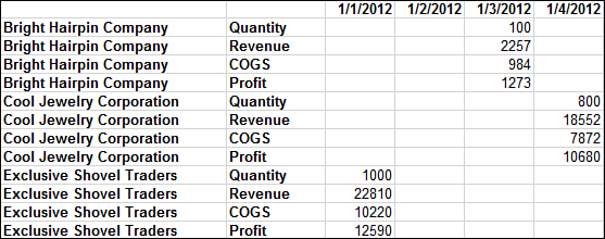
Figure 5.1. Laying out data with dates across the top may make sense when you want to see the data by date, but it can make it more difficult to apply simple formulas or functions.

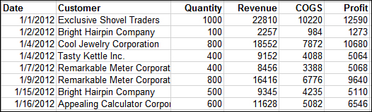
Figure 5.2. Providing a column field for each data type allows you to take full advantage of Excel’s functionality, such as pivot tables and functions like VLOOKUP and SUMIF.

Adjusting Calculation Settings

By default, Excel calculates and recalculates whenever you open or save a workbook or make a change to a cell used in a formula. At times, this isn’t convenient—such as when you’re working with a very large workbook with a long recalculation time. In times like this, you will want to control when calculations occur.

The Calculation group on the Formulas tab has the following options:

• Calculation Options—Has the options Automatic, Automatic Except for Data Tables, and Manual

• Calculate Now—Calculates the entire workbook

• Calculate Sheet—Calculates only the active sheet

The calculation options under File, Options, Formulas include the same Calculation Options as the preceding list, but the Manual option allows you to turn on/off the way Excel recalculates a workbook when saving it.

Viewing Formulas Versus Values

You can’t tell the difference between a cell containing numbers and one with a formula just by looking at it on the sheet. To see whether a cell contains a formula, select the cell and look in the formula bar. If the formula bar contains just a number or text, the cell is static. But if the formula bar contains a formula, which always starts with an equal sign (=), as shown in Figure 5.3, you know the value you’re seeing on the sheet is a result of a calculation.

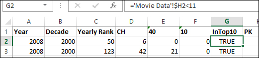
Figure 5.3. The formula bar reveals whether a cell, in this case cell G2, contains a number or a formula.

Another way to view formulas on a sheet is to make them all visible. That is, Excel shows all formulas instead of the calculated values. There are several ways to toggle between viewing values and formulas:

• Press Ctrl+~.

• Go to Formulas, Formula Auditing, Show Formulas on the ribbon.

• Go to File, Options, Advanced and under Display Options for This Worksheet, select Show Formulas in Cells Instead of Their Calculated Results.

If you just want to see what cells have formulas, but don’t need to see the formulas themselves, you can use the Formulas option in the Go to Special dialog box. Press Ctrl+G and click Special to open the dialog box, or go to Home, Editing, Find & Select, Go To Special. Select Formulas and click OK and all formulas on the sheet will be selected, as shown in Figure 5.4.

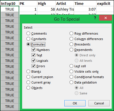
Figure 5.4. Using the Formulas option of the Go to Special dialog box highlights all the formulas on the sheet. Once selected, you can modify the cells, such as ensuring they are protected or applying a fill to them.

Entering a Formula into a Cell

Entering a basic formula is straightforward. Select the cell, enter an equal sign, type in the formula, and press Enter. Typing the formula is very similar to entering an equation on a calculator, with one exception. If one of the terms in your formula is already stored in a cell, you can point to that cell instead of typing in the number stored in the cell. The advantage of this is that if that other cell’s value ever changes, your formula automatically updates.

To enter a formula that includes a pointer to another cell, follow these steps:

1. Select the cell you want the formula to be in.

2. Type an equal sign. This tells Excel you are entering a formula.

3. Type the first number and an operator, as you would on a calculator. There’s no need to include spaces in the formula.

4. Select the cell you want to include in the formula. The cell can even be on another sheet or in another workbook.

5. Press Enter. Excel calculates the formula in the cell.

Of course, there’s no need to have any numbers in a formula. It can consist entirely of cell addresses, as shown in Figure 5.5. The table in the figure calculates the total value of inventory by multiplying the cost (column B) by the quantity (column C). To enter the formula, after typing the equal sign, select the first cell, type an operator, then select the second cell. After pressing Enter, copy the formula down to the other rows using the fill handle.

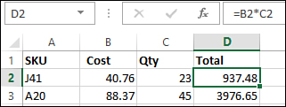
Figure 5.5. Using cell addresses in formulas, instead of values, means the value in cell D2 automatically updates when those other cells, B2 and C2, are updated.

Three Ways of Entering a Formula’s Cell References

After typing the equal sign to start a formula, you have three options for entering the rest of the formula:

• Type the complete formula.

• Type numbers and operator keys, but use the mouse to select cell references.

• Type numbers and operator keys, but use the arrow keys to select cell references.

The method you use depends on what you find most comfortable. Some users consider the first method the quickest because they never have to move their fingers off the main section of the keyboard. For others, using the mouse makes more sense, especially when selecting a large range for use in the formula.

Relative Versus Absolute Formulas

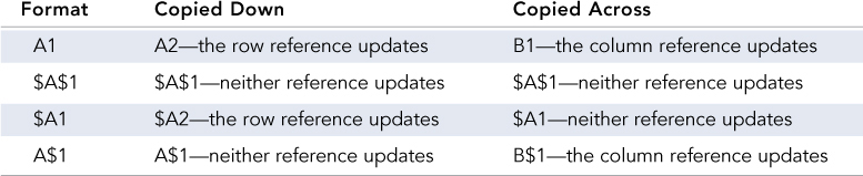
When you copy a formula, such as =B2*C2, down a column, the formula automatically changes to =B3*C3, then =B4*C4, and so on. Excel’s capability to change cell B2 to B3 to B4 and so on is called relative referencing. This is Excel’s default behavior when dealing with formulas, but it might not always be what you want to happen. If the cell address must remain static as the formula is copied, you need to use absolute referencing. This is achieved through the strategic placement of dollar signs ($) before the row or column reference, as shown in Table 5.1.

Table 5.1. Relative Versus Absolute Reference Behavior

Using a Cell on Another Sheet in a Formula

When writing a formula, not all the cells you need to use have to be on the same sheet. As a matter of fact, it might be a better design to have different types of information on different sheets and then pull them together on one sheet using formulas. For example, if you have to periodically import data from another source, instead of possibly messing up the layout of your calculation table by sharing the sheet with the imported data, import the table to a separate sheet and use linked formulas to reference the required cells. Another use could be a lookup table that you allow users to update, but the sheet with the calculations is protected, allowing users to only view that information, not edit it.

To reference a cell on another sheet, navigate to the sheet and then select the cell, as you would if the cell were on the same sheet as the formula. If you have more cells to select, enter your operator and continue to select cells, returning to the formula sheet if needed. If the last cell you need is on a different sheet, press Enter when you are done and Excel returns you to the sheet with the formula.

Figure 5.6 shows a sales sheet that calculates the tax for each record (row). Instead of placing the tax rate in the formula itself, it is placed in another cell on a sheet named Lookups. The tax formula uses an absolute reference to the tax rate cell (Lookups!$B$1), but a relative reference to the cost of the item (D2), as shown in Figure 5.6. When the formula is copied down, all records reference not only the tax rate cell, but their own item cost. And, if the tax rate needs to be modified, you only have to change it in the one cell (Lookups!$B$1) to update all the records.

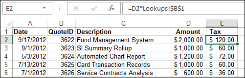
Figure 5.6. A separate sheet is often used to store lookup values, like the Lookups sheet in this formula. This is a good idea because it makes layout changes to the data sheet easier.

Using R1C1 Notation to Reference Cells

The default setting in Excel is A1 notation. R1C1 notation is another reference style for cells. To turn it on, go to File, Options, Formulas and in the Working with Formulas section, select R1C1 Reference Style. When you do this, your sheet column headers change from letters to numbers, as shown in Figure 5.7.

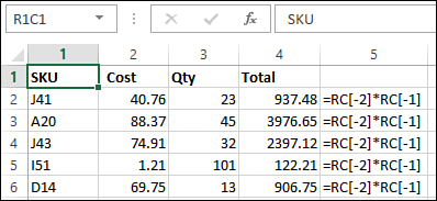
Figure 5.7. R1C1 notation is very different from the A1 reference style.

Instead of A1 in the Name box when you select the top leftmost cell on a sheet, you see R1C1, which stands for Row 1 Column 1, the reverse of A1 style where we have column (A) then row (1). There are three basic rules to R1C1 notation:

• If there’s no number next to the letter, then it’s the current row or column.

• If the number is right next to the letter, then it’s an absolute reference.

• If there are brackets around the number, then it’s a relative reference.

In R1C1 notation, the reference RC refers to the current cell. If the R or C does not have a number next to it, then the reference is to the row or column in which the formula appears. For example, if you type =RC5 in cell B26, when you revert to A1 style, =$E26 now appears in the cell. The R does not have a number next to it, so it refers to the row in which the formula is typed (26). Notice the column reference in this example is absolute (has a $). That’s because in the R1C1 notation, the number (5) appears right next to the C. Whereas in A1 notation you use a dollar sign ($) to denote absolute referencing, the lack of anything separating the letter and number denotes absolute referencing in R1C1 style.

To indicate relative referencing in R1C1 style, you modify RC by adding or subtracting the number of rows or columns representing the location of the cell in reference to the active cell. Keep in mind these rules for relative referencing:

• The numbers must be enclosed in square brackets.

• When referring to a cell above or to the left of the active cell, the number is negative.

• When referring to a cell below or to the right of the active cell, the number is positive.

For example, if you have a formula in cell G8 and use the reference R[-1]C[3], you are referring to a cell one row above and 3 columns to the right of G8, which is J7.

In Figure 5.7, all the formulas are the same because the formula is based off the cell the formula is in. Note the formulas shown are actually the formulas in the Total column. The formula multiplies the value in the cell two columns to the left (Cost) by the value one column to the left (Qty) of the formula cell (Total). Both references are to a cell in the same row as the formula, so there is no number by the row reference.

Using F4 to Change the Cell Referencing

When you type in a formula and select a cell or range, Excel uses the relative reference. If you need the absolute reference, you will probably either type in the address manually or go back and change the address after you are done with the whole formula. Another option is to change the reference to what you need while typing in the formula. You can do this by pressing the F4 key right after selecting the cell or range. Each time you press the F4 key, it changes the cell address to another reference variation, as shown in Figure 5.8.

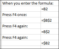
Figure 5.8. Use F4 to toggle through the variations of relative to absolute referencing.

For example, to change the cell address in a formula to a column fixed reference as you type it in, follow these steps:

1. Select the cell you want the formula to be in.

2. Type an equal sign.

3. Type the first number and operator, as you would on a calculator.

4. Select the cell you want to include in the formula.

5. Press F4 once and the address changes to absolute referencing. Press F4 again and it becomes a Row Fixed Reference. Press F4 a third time and it becomes a Column Fixed Reference.

6. Press Enter. Excel calculates the formula in the cell.

Mathematical Operators

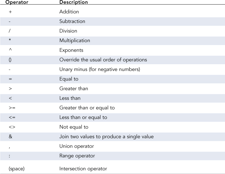
Excel offers the mathematical operators listed in Table 5.2.

Table 5.2. Mathematical Operators

Order of Operations

Excel evaluates a formula in a particular order if it contains many calculations. Instead of calculating from left to right like a calculator, Excel performs certain types of calculations, such as multiplication, before other calculations, such as addition.

You can override this default order of operations using parentheses. If you don’t, Excel applies the following order of operations:

1. Unary minus

2. Exponents

3. Multiplication and division, left to right

4. Addition and subtraction, left to right

For example, if you have the formula

=6+3*2

Excel returns 12, because first it does 3*2, then adds the result (6) to 6. But, if you use parentheses, you can change the order:

=(6+3)*2

produces 18 because now Excel will do the addition first (6+3) and multiply the result (9) by 2.

Copying a Formula to Another Cell

You can use four ways to enter the same formula in multiple cells:

• Copy the entire cell and paste it to the new location.

• Enter the formula in the first cell and then use the fill handle to copy the formula.

• Preselect the entire range for the formula. Enter the formula in the first cell and press Ctrl+Enter to simultaneously enter the formula in the entire selection.

• Define the range as a Table. Excel automatically copies new formulas entered in a Table. See the section “Inserting Formulas into Tables” for more information.

Copying a Formula Using the Fill Handle

This method is useful if you need to copy your formula across a row or down a column. To copy a formula by dragging the fill handle, follow these steps:

1. Select the cell you want the formula to be in.

2. Type the formula in the first cell.

3. Press Ctrl+Enter to accept the formula and keep the cell as your active cell. If you press Enter instead, that’s fine—just reselect the cell.

4. Click and hold the fill handle, which looks like a little black square in the lower-right corner of the selected cell. When the cursor is positioned correctly, it turns into a black cross, as shown in Figure 5.9.

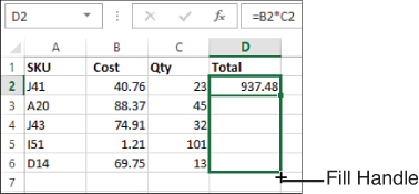
Figure 5.9. Clicking and dragging the fill handle is a quick way to copy a formula a short distance.

5. Drag the fill handle to the last cell that needs to hold a copy of the formula.

6. Release the mouse button. The first cell is copied to all the cells in the selected range.

Copying a Formula by Using Ctrl+Enter

If you have a large range to copy a formula into, and the range isn’t a single column or single row, this method might be useful. It copies the formula into the columns and/or rows of the selection, such as a rectangle or even a selection of noncontiguous cells. To copy a formula using Ctrl+Enter, follow these steps:

1. Select the range, or noncontiguous cells, you want the formula to be in.

2. Type the formula in the first cell, ensuring your cell referencing is correct.

3. Press Ctrl+Enter. Excel copies the formula to all cells in the selected range.

Copying Formulas Rapidly Down a Column

If you need to copy a formula into just a few rows, using the fill handle is fine. But if you have several hundred rows to update, you could zoom right past the last row. And if you have thousands of rows, using the fill handle can take quite some time.

One solution is to copy the formula, select the range, and paste the formula into the range. But it can still be a bit tricky to select the entire range you need to paste to.

If you have a data set without any completely blank rows, you can double-click the fill handle and have it quickly fill the formula down the column to the last row of the data set.

To quickly fill the formula down the column to the last row of the data set, follow these steps:

1. Enter your formula in the first cell of the column.

2. Verify that your data set is contiguous without any blank rows or columns. To do this, select the cell from step 1 and press Ctrl+A. Excel selects all the cells of the data set until it runs into a blank row and column. If you see any blank columns or rows interfering with the desired selection, add some temporary text and then try the selection again.

3. Once you’ve verified that the data set is contiguous, place your cursor on the fill handle until it turns into a black plus sign, as shown in Figure 5.9.

4. Double-click and the formula will be copied down the sheet until it reaches the end of the data set (a fully blank row).

Using Names to Simplify References

It can be difficult to remember what cell you have a specific entry in, such as a tax rate, when you’re writing a formula. And if the cell you need to reference is on another sheet, you have to be very careful writing out the reference properly, or you must use the mouse to go to the sheet and select the cell.

It would be much simpler if you could just use the word TaxRate in your formula—and you can, by applying a Name to the cell. After a Name is applied to a cell, any references to the cell or range can be done by using the Name instead of the cell address. For example, where you once had =B2*$H$1, you could now have =B2*TaxRate, assuming H1 is the cell containing the tax rate.

There are only a few limitations to remember when creating a Name:

• The Name must be one word. You can use an underscore (_), backslash (), or period (.) as spacers.

• The Name cannot be a word that might also be a cell address. This was a real problem when people converted workbooks from legacy Excel to Excel 2007 or newer because some names, such as TAX2009, weren’t cell addresses before. Now in Excel 2007 and newer, such Names cause problems when opening a legacy workbook. So Name carefully!

• The Name cannot include any invalid characters, such as ? ! or -. The only valid special characters are the underscore (_), backslash (), and period (.).

• Names are not case sensitive. Excel will see “sales” and “Sales” as the same name.

• You should not use any of the reserved words in Excel. These are Print_Area, Print_Titles, Criteria, Database, and Extract.

Applying and Using a Name in a Formula

To apply a Name to a cell, select the cell, type the Name in the Name box, and press Enter. As long as the Name has not been applied to another cell in the workbook, it replaces the cell address of the selected cell. But if the Name has been applied elsewhere in the workbook, Excel takes you to that cell.

To apply a name to a cell and then use the name in a formula, follow these steps:

1. Select the cell or range you want to apply the Name to.

2. In the Name field, type in the Name, as shown in Figure 5.10.

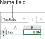
Figure 5.10. After you select a cell or range, you can type a Name for it in the Name field.

3. Press Enter for Excel to accept the Name.

4. Go to the cell containing the formula that should reference the Name.

5. Replace the cell or range address with the Name you just created, or type in a new formula from scratch using the Name where you would use the cell or range address, as shown in Figure 5.11.

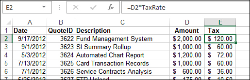
Figure 5.11. Using Names can simplify entering formulas.

If you can’t remember the Name assigned to a range, you can look it up by clicking the drop-down in the Name field or by selecting Formulas, Defined Names, Use in Formula, which opens up a drop-down of available Names. You can also go to Formulas, Defined Names, Name Manager, which not only lists the defined Names but shows the range they apply to.

Global Versus Local Names

Names can be global, which means they are available anywhere in the workbook. Names can also be local, which means they are available only on a specific sheet. With local Names, you can have multiple references in the workbook with the same name. Global Names must be unique to the workbook.

The Name Manager dialog box (shown in Figure 5.12 and found in the Defined Names group on the Formulas tab), lists all the Names in a workbook, even a Name that has been assigned to both the global and local levels. The Scope column lists the scope of the Name, whether it is the workbook or a specific sheet such as Sheet1. When you create a Name, by default it is global. To make the Name local, you have to include the sheet name followed by an exclamation point (!) before typing the Name. If the sheet name is more than one word, then you have to wrap the sheet name in single quotes. For example, if the sheet name is “SD Sales” and you’re creating the TaxRate name to use just on that sheet, the Name you type would be: ‘SD Sales’!TaxRate.

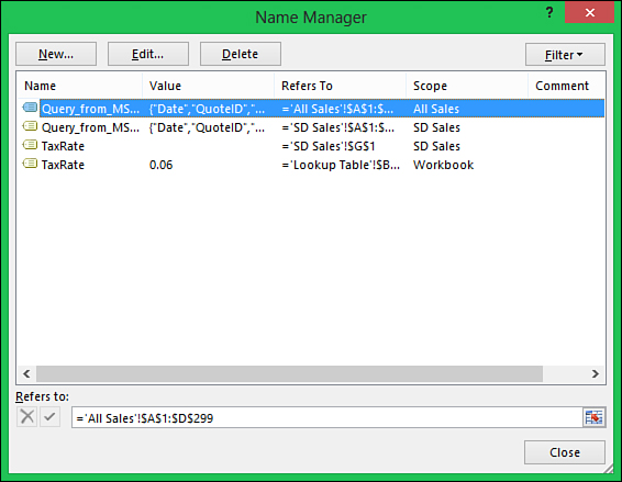
Figure 5.12. The Name Manager dialog box lists all local and global names.

Inserting Formulas into Tables

When your data has been defined as a Table, Excel automatically copies new formulas created in adjacent columns down to the last row in the Table.

To add a new calculated column to a Table, follow these steps:

1. Type a field header in row 1 of the column adjacent to the rightmost column of the Table. Excel extends any Table formatting to the new column.

2. Select the first data cell in the column. This is cell H2 in Figure 5.13.

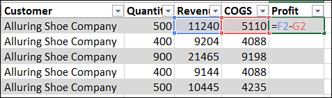
Figure 5.13. Type a formula in the first cell of a Table column and Excel copies it down the rest of the column. Note that if you select the columns instead of typing in the cell references, your resulting formula will look quite different.

3. Type your formula for the selected cell.

4. Press Enter and Excel copies the formula down the column.

After entering the formula, a lightning bolt drop-down appears by the cell. If you don’t want the automated formula copied, select Undo Calculated Column or Stop Automatically Creating Calculated Columns.

Using Table Names in Table Formulas

Names are automatically created when you define a Table. A name, or a specifier, for each column and the entire Table is created. Just like you can use Names to simplify references in your standard formulas, you can use these names to simplify references to the data in your Table formulas. A formula using [@Quantity] is easier to understand than E2.

To create a Table formula using column specifiers instead of cell addresses, you can type in the column name preceded by @ and surrounded by square brackets or you can use the mouse or keyboard to select the desired cell in the Table. To add a new calculated column to a Table, follow these steps:

1. Type a field header in row 1 of the column adjacent to the rightmost column of the Table. Excel extends any Table formatting to the new column.

2. Select the first data cell. This is cell H2 in Figure 5.14.

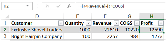
Figure 5.14. The use of specifiers in Table formulas makes it much easier to interpret what fields are used in the calculation.

3. Enter your formula. Instead of typing in cell addresses, use the keyboard or mouse to select the cells. You will notice that column specifiers appear instead of cell addresses.

4. Press Enter and Excel copies the formula down the column.

After entering the formula, a lightning bolt drop-down appears by the cell. If you don’t want the automated formula copied, select Undo Calculated Column or Stop Automatically Creating Calculated Columns.

In Figure 5.14, look at the formula in the formula bar. Notice the column specifiers are preceded by @. This is to specify that the formula is referring to the value of the specifier in that column. If the @ is dropped, then the formula would be referring to the entire column. For more information on @ and other specifiers, see the next section “Writing Table Formulas Outside the Table.”

Writing Table Formulas Outside the Table

To find the name of the Table, select a cell in the Table and go to Table Tools, Design, Properties. The name of the Table appears in the Table Name field. You use this name in formulas to reference the entire Table.

In addition to the Table and column specifiers, Excel provides five more to make it easier to narrow down a particular part of a Table:

• #All—Returns all the contents of the Table or specified column

• #Data—Returns the data cells of the Table or specified column

• @ (This Row)—Returns the current row

• #Headers—Returns all the column headers or that of a specified column

• #Totals—Returns the total rows or that of a specified column

To access these specifiers from a drop-down, you must first type the Table name followed by the left square bracket. After the bracket is entered, a drop-down of all specifiers appears, as shown in Figure 5.15. For example, to return the sum of the entire Profit column in Table1, the formula would be:

=SUM(Table1[Profit])

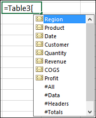
Figure 5.15. You can manually type in a specifier, or when the drop-down appears, arrow down to the desired specifier and click Tab to add it to the formula.

If you wanted to return the profit made from a specific company, Alluring Shoe Company, from the same Table, the formula would be:

=SUMIF(Table1[Customer],”Alluring Shoe Company”,Table1[Profit])

Another user would not need to see the Table. As long as the Table name and field name are known, the user can write any desired formula.

The following are rules for writing formulas that refer to Tables:

• The reference to the Table must start with the Table name. If the formula is within the Table itself, you can omit the Table name.

• Specifiers, such as a column name or the total row, must be enclosed in square brackets, like this: TableName[Specifier].

• If using multiple specifiers, each specifier must be surrounded by square brackets and separated by commas. The entire group of specifiers used must be surrounded by square brackets, like this: TableName[[Specifier1], [Specifier2]].

• If no specifiers are used, the Table name refers to the data rows in the Table. This does not include the headers or total rows.

• The @ (This Row) specifier must be used with another specifier, like this: TableName[[@Specifier]].

Figure 5.16 shows examples of using specifiers.

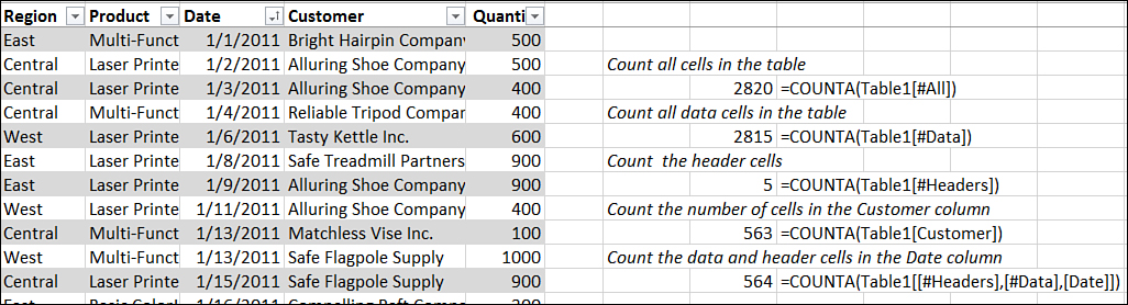
Figure 5.16. Column I has examples of using specifiers to return Table information.

Using Array Formulas

An array holds multiple values individually in a single cell. An array formula allows you to do calculations with those individual values.

It’s hard to imagine, but three keys on your keyboard can turn the right formula into a super formula. Three keys can take 10,000 individual formulas and reduce them to a single formula. These three keys are Ctrl+Shift+Enter. Enter the right type of formula in a cell, but instead of just pressing Enter, press Ctrl+Shift+Enter and the formula becomes an array formula, also known as a CSE formula.

For example, with an array formula you can do the following:

• Multiply corresponding cells together and return the sum or average, as shown in Example 2.

• Return a list of the top nth items in a list, while calculating the value by which you are judging their rank, as shown in Example 3.

• Sum (or average) only numbers that meet a certain condition, such as falling between a specified range.

• Count the number or records that match multiple criteria.

You can tell if a formula is an array formula because it’s surrounded by curly braces ({}). These braces are not typed in. They appear after pressing Ctrl+Shift+Enter. If you edit the formula, the braces will go away and you’ll have to press the CSE combination to get them to come back, or press Esc to exit the cell and undo any changes.

Example 1

Look at Figure 5.17. The ROW function returns the row number of what is in the parentheses. When you have a range, such as $1:$10, the function holds all the numbers 1 to 10. In columns A and B, you see the result of a normally entered ROW function looking at rows 1:10—1s all the way down because the formula can only return the first value it holds. In columns C and D, you see the same formula, but entered as an array formula. This time, you can see each value held in the function—the numbers 1 through 10.

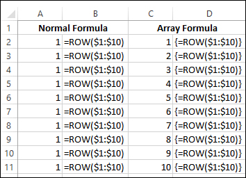
Figure 5.17. Normally, the formula in B2:B11 would return only a single value. But enter the same formula as an array formula, and range C2:C11 shows the individual values held in the array formula.

Excel returns the value corresponding to the cell’s position in the entire range the array is applied to. To let Excel know what the range is, you select the range before you type the formula in. In this case, C2:C11 was selected, the formula typed into C2, then CSE was pressed, applying the array to the range.

Example 2

Figure 5.18 goes to the next step, multiplying each value in the array by 2, as shown in columns H and I. Cell H10 includes the SUM function in the array formula, which not only multiplies each value in the array by 2 but also adds the results. Imagine if you had a sheet with 10,000 quantities and prices. Instead of multiplying each row into a new column and then summing that column, you just have one cell that does the entire calculation. And because you have fewer formulas, the workbook is smaller.

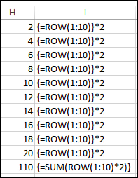
Figure 5.18. The array formula in cell H11 multiplies each value in the array and sums the results.

Example 3

An array formula can also calculate and return multiple values. These values are placed within the range selected before entering the formula.

For example, if you want to return the region, product, and date of the top three revenue generators for the data in Figure 5.19, use a formula like this (explained in more detail after the figure):

=INDEX(A1:A46 & “-” & B1:B46 & “ on “ &

TEXT(C1:C46,”mm/dd/yy”),MATCH(LARGE(D2:D46*E2:E46,{1;2;3}),(D1:D46*E1:E46),0))

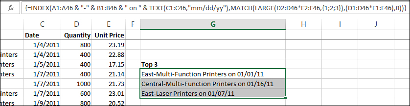
Figure 5.19. An array formula can be used to return multiple values, such as the top three revenue makers.

1. Look for the three largest revenues at the same time they’re being calculated, like this:

LARGE(D2:D46*E2:E46,{1;2;3})

LARGE is a function that returns the nth largest value in a range, which we are creating by multiplying corresponding values in columns D and E (D2*E2, D3*E3, and so forth). In this case, we are looking for the top three items and place 1;2;3 in curly braces. By placing the numbers manually in curly braces separated by semicolons (;), we’re identifying them as an array.

2. Now that we have the top three values, we have to locate them within the range, like this:

MATCH(LARGE(D2:D46*E2:E46,{1;2;3}),(D1:D46*E1:E46),0)

MATCH returns the row numbers of the calculated revenues by matching their location within an array of the calculated revenues. The 0 tells the function we need an exact match to the values.

3. The formula now holds the rows that the three largest values are found in. The INDEX function is then used to look up and return the desired details from those rows.

4. After you select three cells where you want the results of the formula placed, type the entire formula and enter it by pressing Ctrl+Shift+Enter. Excel copies the formula down to each of the three cells. The first cell returns the first answer in the calculated array, the second cell returns the second value in the calculated array, and the third cell returns the third value.

When an array formula is holding more than one calculated value, you must select a range at least the size of the most values it is returning before entering it and pressing the CSE combination. If the range selected is too small, only some of the values will be returned. If the range selected is too large, an error will appear in the extra cells. Because you have the same formula in multiple cells, the workbook is smaller; Excel has to track only a single formula.

Editing Array Formulas

Following are a few rules to use when editing multicell array formulas:

• You cannot edit just one cell of the array formula. A change made to one cell affects them all.

• You can increase the size of the range but not decrease it. To decrease it, you must delete the formula and reenter it.

• You cannot move just a part of the range, but you can move the entire range.

• The range must be continuous—you cannot insert blank cells within it.

Deleting Array Formulas

You cannot delete just one cell of a multicell array formula. The entire range containing the array formula must be selected before you can delete it. The message “You Cannot Change Part of an Array” will appear if you try to delete just a portion of the range containing the formula. You can use Go to Special, Current Array to select the entire array or select one cell in the array, press Backspace, then Ctrl+Shift+Enter and this will clear all the cells in the array.

If you need to resize an array to be smaller, you will have to delete and reenter it. To select an entire array formula and delete it, follow these steps:

1. Select a cell in the array formula.

2. Press Ctrl+G to bring up the Go To dialog box.

3. Click the Special button in the lower-left corner of the dialog box.

4. Select Current Array and click OK.

5. Press Delete on the keyboard to delete the entire array formula range.

Converting Formulas to Values

Formulas take up a lot of memory, and the recalculation time can make working in a large workbook a hassle. At times, you need a formula only temporarily; you just want to calculate the value once and won’t ever need to calculate it again. You could manually type the value over the formula cell, but if the result is a long number, or if you have a lot of calculation cells, this isn’t convenient. You could copy the range then do a Paste Special, Values, but there’s a faster option you can access from a special right-click menu. To access the menu and quickly convert formula to their values, follow these steps:

1. Select the range of formulas.

2. Place your cursor on the right edge of the dark border around the range so that it turns from the white plus sign to four black arrows, as if you were going to move the range to a new location.

3. While holding your right mouse button down, drag the range to the next column and then back to the original column.

4. Let go of the right mouse button.

5. From the context menu that appears, shown in Figure 5.20, select Copy Here as Values Only.

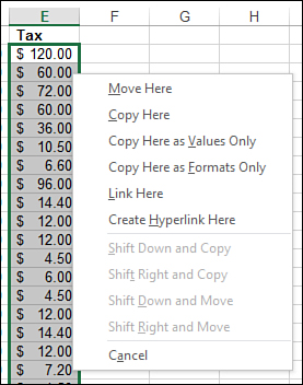
Figure 5.20. By placing the cursor on the range’s border, holding down the right mouse button and dragging to and fro, a hidden menu appears with various options to apply to the range.

Troubleshooting Formulas

It can be frustrating to enter a formula and have it either return an incorrect value or an error. An important part of solving the problem is to understand what the error is trying to tell you. After you have an idea of the problem you’re looking for, you can use several tools to look deeper into the error.

Error Messages

After entering a formula, you may run into one of the following errors:

• #DIV/0!—Occurs when a number is divided by zero.

• #N/A—Occurs when a value isn’t available in the formula; for example, if you’re doing a lookup function and the lookup value isn’t found.

• #NAME?—Occurs when a formula includes unrecognizable text.

• #NULL!—Occurs when an intersection is specified but the areas do not intersect or if a range operator is incorrect. For example, if you entered =SUM(A1:A10 B1:B10), you would get the error because the comma separating the ranges is missing. The correct formula is =SUM(A1:A10,B1:B10).

• #NUM!—Occurs when there is an invalid numeric value in a formula or function.

• #REF!—Occurs when a cell reference isn’t valid, for example, if the cell has been deleted. This can be difficult to trace because the #REF can occur within the formula itself—for example, =#REF*A2—and there’s no direct way to trace back to the original reference.

• #VALUE!—Occurs when trying to do math with nonnumeric data; for example, D1+D2 will return the error if cell D1 is the column header.

• ######—This isn’t really an error. It can occur if the column width is not wide enough for the formula result or if you’re trying to subtract a later date from an earlier date (you can’t have a negative date).

The initial help provided by Excel may help trace the problem. When an error cell is selected, an exclamation icon appears. When you click on the icon, a list of options appears.

The first item in the list is a brief description of the issue, so this will change depending on the error. After that, Excel offers four troubleshooting options:

• Help on This Error—Opens the Excel Help dialog box to find more information on troubleshooting formulas.

• Show Calculation Steps—Opens the Evaluate Formula dialog box. See the “Using the Evaluate Formula Dialog Box” section later in this chapter for more information.

• Ignore Error—Causes the error icon to disappear. It reappears if the formula is edited.

• Edit in Formula Bar—Puts you in Edit mode, with your cursor in the formula bar. The cells used in the formula, if on the same sheet, are highlighted so you can see what ranges are being used.

At the bottom of the list, is a link to the Excel Options dialog box, Formulas section, where you can modify how Excel interacts with you when it comes to errors.

Additional troubleshooting options are available in the Formula Auditing group on the Formulas tab.

Using Trace Precedents and Dependents to See What Cells Affect or Are Affected By the Active Cell

When you select a cell containing a formula and press F2, you enter Edit mode and Excel highlights any cells on the sheet that are used by the formula. But it doesn’t highlight the cells on other sheets. To do that and more, use the trace precedent and trace dependent auditing arrows.

Use the formula auditing arrows found on the Formulas tab in the Formula Auditing group if you have a cell you want to trace, whether it’s to locate other cells used in that cell’s formula or what cells reference the selected cell. Just select the cell in question and click a trace button.

There are two types of auditing arrows:

• Trace Precedents—If the selected cell contains a formula, blue arrows point to the cells used by the formula.

• Trace Dependents—If the selected cell is used in a formula in another cell, red arrows point to the cell containing that formula.

When you click one of the trace buttons, arrows appear linking the cell to other cells that are directly connected to it, as shown in Figure 5.21. Click the trace button again and you will get the next level of cell connections. You can continue to click the button and Excel continues adding tracing arrows to the sheet.

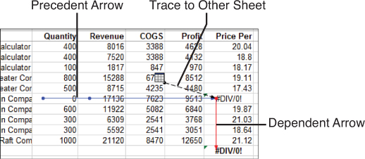
Figure 5.21. Use the Trace Precedents and Trace Dependents buttons to locate links to the selected cell, including links to other sheets.

If the connecting cell is on another sheet, Excel displays a dashed arrow pointing to a sheet icon, as shown in Figure 5.21. If you double-click the line (make sure your cursor is a white arrow, not a white plus), the Go To dialog box appears, listing every cell containing a link to the selected cell. You can then double-click one of the listed items in the dialog box and jump directly to the linked cell.

To clear all the arrows, select Formulas, Formula Auditing, Remove Arrows. There is no way to go back just one level or remove one type of arrow.

Using the Watch Window to Track Formulas on Other Sheets

The Watch Window found in the Formula Auditing group of the Formulas tab allows you to watch a cell update as you make changes that will affect it. This can be useful when you have formulas that span multiple sheets and you need to watch a cell on one sheet while you make changes to another. You can double-click a cell in the Watch Window to jump to that cell.

To watch a formula update on another sheet, follow these steps:

1. Select Formulas, Formula Auditing, Watch Window. The Watch Window dialog box opens.

2. Click Add Watch to open the Add Watch dialog box.

3. Select the cell you want to watch update and click Add.

4. Repeat steps 2 and 3 for any additional cells that you want to monitor.

5. Leave the Watch Window open (you can drag it out of the way) and make changes to cells that will affect the watched cells.

6. Whether directly linked or not, if the watched cells are in any way affected by the changes you make, the Watch Window updates to reflect the new value of the cell.

Using the Evaluate Formula Dialog Box

If you want to watch how Excel calculates each part of a formula, you can use Formulas, Formula Auditing, Evaluate Formula.

The Evaluate Formula dialog box, shown in Figure 5.22, has three buttons you can use to investigate a formula. The buttons work only on the underlined portion of the formula:

• Evaluate—Replaces the underlined portion of the formula with the value.

• Step In—Displays the actual contents of a cell if the underlined portion is a cell address. This may be a value or a formula. If it’s a formula, you have the option to continue stepping in until it is resolved.

• Step Out—Returns to the previous level of evaluation.

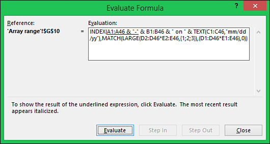
Figure 5.22. The Evaluate Formula dialog box is just one tool for troubleshooting formula errors. With this tool, you can watch the results as Excel calculates each portion of a formula.

You can continue to evaluate a formula until it is completely resolved.

To see how Excel is calculating each part of a formula, follow these steps:

1. Select the cell with the formula to evaluate.

2. Select Formulas, Formula Auditing, Evaluate Formula. The formula appears in the evaluation window with some part of it underlined, as shown in Figure 5.22.

3. Click the Step In button if it is activated. If it isn’t, skip to step 8. A new section appears in the window, showing the result of the underlined portion.

4. Repeat steps 4 and 5 if the Step In button is still active.

5. When the Step In button is no longer active, click the Step Out button to return to the previous level. Each click of the button returns you to the previous level.

6. Click the Evaluate button and Excel evaluates the underlined portion, replacing it in the formula with the returned or calculated value.

7. Continue to click Evaluate or Step In to watch the formula calculate.

8. Excel is done with the evaluation when only the calculated value appears in the Evaluation field. You can either click Restart to go through the steps again, or click Close to return to Excel.

Evaluating with F9

With the Evaluate Formula dialog box, you have to evaluate the formula in the order that Excel calculates the formula. If you want to jump directly to a portion of the formula, you can skip the Evaluate Formula dialog box and instead just highlight that formula portion and press F9 to evaluate to its value.

You should keep two things in mind when using F9 to evaluate a formula:

• When highlighting the portion to evaluate, you must be careful to select the entire portion, including any relevant parentheses.

• You must press Esc to leave the cell. If you don’t, Excel replaces your formula with the value you just evaluated to.