6. Using Functions

A function is like a shortcut for using a long or complex formula. If you’ve ever summed cells like this: =A1+A2+A3+A4+A5, you could have instead used the SUM function like this: =SUM(A1:A5). Excel offers more than 400 functions. These include logical functions, lookup functions, statistical functions, financial functions, and more.

This chapter shows you how to look up functions available in Excel and reviews some functions helpful for everyday use. Another useful tool, Goal Seek, is also introduced.

Breaking Down a Function

A function consists of the name used to call it and might or might not include arguments, which are variables used in the calculation. In the formula =SUM(A1:A5), SUM is the function and A1:A5 is the argument.

Normally, the syntax of a function is like this:

FunctionName(Argument1, Argument2, ...)

But there are some functions that have no arguments or the argument is optional. There are a few rules to keep in mind when using functions:

• Arguments must be entered in the order required by the function.

• Arguments must be separated by commas.

• Arguments can be cell references, numbers, logicals, or text.

• Some arguments are optional. Optional arguments are placed after the required ones.

• If you skip an optional argument to use one after it, you still have to place a comma for the one you skipped.

• Some functions, such as NOW(), do not require arguments, but the parentheses must still be included in the formula.

Finding Functions

You can always search Excel’s Help to find a function, but you might get more than just the function information you’re looking for. Instead, narrow down the results by using tools provided specifically for searching functions.

The Formulas tab has a Function Library group with drop-downs grouped by function type. Selecting any function listed in a drop-down opens it up in the Formula Wizard.

If you aren’t sure which function you need, or if you need more help in using a function, there are several ways to open the Insert Function dialog box, which helps you find the required function:

• Select the More Functions link at the bottom of the AutoSum drop-down on the Home or Formulas tab.

• Select the Insert Function link at the bottom of one of the other function library drop-downs on the Formulas tab.

• Click the Insert Function button in the Function Library group on the Formulas tab.

• Click the fx button by the formula bar.

When you click Insert Function, the dialog box shown in Figure 6.1 opens. You can enter a search term in the Search for a Function field or select a category from the drop-down. Results appear in the list box. When you select a function from the list box, the arguments and a brief description of the function appear. When you find the function you want to use, highlight it and click OK. The function appears in the active cell and the Function Arguments dialog box opens, ready to help you fill in the rest of the arguments.

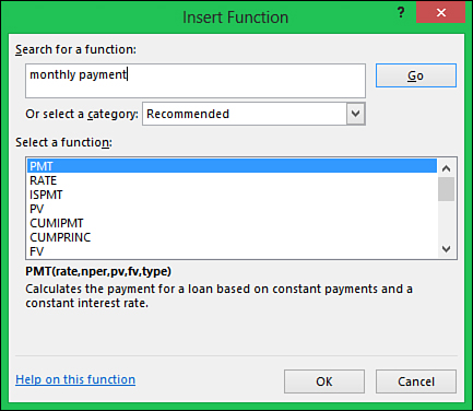
Figure 6.1. The Insert Function dialog box helps search through Excel’s more than 400 available functions.

Entering Functions Using the Function Arguments Dialog Box

Once you’ve entered a function in a cell, the Function Arguments dialog box shown in Figure 6.2 opens. It assists in entering the arguments for the selected function. Other than from beginning with the Insert Function dialog box as explained in the previous section, you can also open the dialog box by selecting a cell with a function already in it and using any of the methods listed in the “Finding Functions” section.

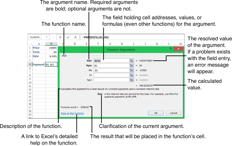
Figure 6.2. The Function Arguments dialog box helps with the arguments of the selected function.

A field exists for each argument. If the function has a variable number of arguments, like the SUM function, a new field is automatically added when needed.

Figure 6.2 shows the PMT function being used to calculate the monthly payment for a loan. The loan amount is in cell B1, the number of months in cell B2, the APR in cell B3. The function is in cell B5. To insert the function and select its arguments, follow these steps:

1. Select the cell that will hold the formula (cell B5).

2. Go to Formulas, Insert Function. In the Search field, type PMT and click Go.

3. PMT should appear in the list of functions. Highlight it and click OK. The Function Arguments dialog box should appear. If the dialog box is covering the values on the sheet (B1:B3), then click the title of the dialog box and drag it out of the way.

4. The first argument is Rate, the interest rate. When you click in the field and look at the description, notice it says this is the interest rate per period. Because your value is the annual rate, you need to divide it by 12. But first, you need to select it on the sheet. Click cell B3 and the cell address will appear in the Rate field with the cursor blinking at the end of it. Type in /12 to get the monthly rate.

5. The second argument is the Nper, number of payments for the loan. First click the field in the dialog box, then select cell B2 on the sheet.

6. Click in the Pv field (present value of the loan) in the dialog box. Before selecting the cell on the sheet, enter a – (a minus sign) so that when you do click the cell on the sheet, you are making the value negative. You do this because of the way the function works. If you didn’t make this value negative, the payment itself would be negative.

7. Fv (future value after the last payment is made) and Type (when the payment is made—1 at the beginning of the period, 0 at the end of the period) are both optional arguments and can be left blank.

8. If you do not see any error messages in the calculated value in the dialog box, click OK to have the cell accept the formula.

Entering Functions Using In-Cell Tips

If you are already familiar with the function you need, you can begin typing it in the cell or formula bar directly. After you enter an equal sign and select the first letter of the function, Excel drops down a list of possible functions, narrowing down the list with each letter entered. You can also select from the list using the arrow and Tab keys.

After the function is selected, an in-cell tip appears, as shown in Figure 6.3. The current argument will be in bold. Optional arguments appear in square brackets. If you want to use the Function Arguments dialog box, press Ctrl+A after typing the function name in the cell. For more help with the function, click the function name in the tip, and Excel’s detailed Help file for the function appears.

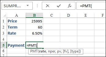
Figure 6.3. If you’re already familiar with the function, you can use the in-cell help to guide you in filling out the arguments.

To type a function, such as SUM, directly into a cell, follow these steps:

1. Select the cell that will hold the formula.

2. Type an equal sign.

3. Begin typing the name of the function. When the drop-down list appears, you can continue typing or scroll the list to highlight the function and press Tab.

4. Enter the first argument. The argument can be a cell address (you can type it in or select it on the sheet), a value, or a formula.

5. If there is another argument, type a comma and then enter the next argument. Repeat this step for each argument. As you enter each argument, notice that the argument becomes bold in the in-cell tip, showing you your position in the function.

6. When you’re finished entering all the arguments, type the closing parenthesis and press Enter or Tab for the cell to accept the formula.

Using the AutoSum Button

Excel provides one-click access to the SUM function through the AutoSum button found under Home, Editing and Formulas, Function Library. You can apply the AutoSum function to a range of cells in a variety of ways:

• Select a cell adjacent to the range and click the AutoSum button.

• Highlight the range including the adjacent cell where you want the formula placed, and then select the AutoSum button.

• If you need to sum multiple ranges, select the entire table, including the adjacent row or column where you want results to appear, and then click the AutoSum button.

Unless you select the range you want to calculate, Excel guesses which cells you are trying to sum and highlights them. If the selection is correct, press Enter to accept the solution. If the selection is incorrect, make the required changes and then press Enter to accept the solution.

You should keep an eye out for a couple of things when using the AutoSum function:

• Be careful of numeric headings (like years) when letting Excel select the range for you. Excel cannot tell that the heading isn’t part of the calculation range, and you need to correct the selection before accepting the formula.

• Excel looks for a column to sum before summing a row. In Figure 6.4, the default selection by Excel is the numbers above the selected cell, instead of the adjacent row of numbers.

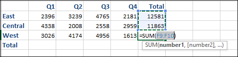
Figure 6.4. Excel defaults to calculating columns before rows. I wanted to sum the West data, but Excel selects the totals from East and Central instead.

SUM Rows and Columns at the Same Time

You can SUM multiple ranges at the same time, including rows and columns. In Figure 6.5, the totals in column F and row 6 were all calculated at the same time. This was done by selecting the entire table, including the Total row and column before clicking the AutoSum button. You could also have a single row and column selection, for example, just Q1 (column B) and East (row 3) data. To do so, follow these steps:

1. Select B3:B6.

2. While holding down the Ctrl key, select B3:F3.

3. Click the AutoSum button.

4. Excel calculates and inserts the corresponding totals in the total cells.

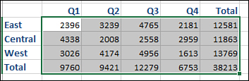
Figure 6.5. Excel is smart enough to determine that you want to sum each individual row and column.

Other Auto Functions

The default action of the AutoSum button is the SUM function, but several other functions are available. To access these other functions, click the drop-down arrow:

• Sum—Adds the values in the selected range (the default action)

• Average—Averages the values in the selected range

• Count Numbers—Returns the number of cells containing numbers

• Max—Returns the largest value in the selected range

• Min—Returns the smallest value in the selected range

These other options work on a range in the same way as the SUM function, but you have to select them from the drop-down, whereas with SUM, you can just click the button.

Using the Status Bar for Quick Calculation Results

If you just need to see the results of a calculation and not include the information on a sheet, Excel offers six quick calculations, listed in Figure 6.6, that appear in the status bar when the data is selected.

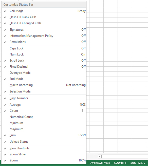
Figure 6.6. You can modify the status bar to show the results of calculations done to selected data.

To see the list of functions and be able to edit the values shown in the status bar, you must first select some data on a sheet. Next, right-click on the status bar and the Customize Status Bar menu, shown in Figure 6.6, appears. You can toggle the check mark next to the functions you want to show or hide in the status bar. Once you have selected the functions you want, whenever you select data, the resulting calculations will appear in the status bar.

Using Quick Analysis for Column Totals

When you select multiple adjacent cells, the Quick Analysis icon, shown in Figure 6.7, appears in the lower-right corner of the selection. Click on the icon, select TOTALS and various quick calculations appear. You can use the arrows on the left and right side of the icons to scroll through the list. Once you find the calculation you want, click on it and the calculated values will be placed at the bottom of each column in your range.

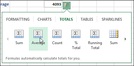
Figure 6.7. The Quick Analysis tool can be used to calculate a column, but not a row.

Using Lookup Functions to Match a Value and Return Another

This section reviews some of the methods available for returning a value by looking up another. There are functions that can return a value dependent on its position in a list or return a value in the same row as a match. You can even combine multiple functions to return a value by looking up and matching multiple variables.

In the function’s syntax, an argument in square brackets is an optional argument.

CHOOSE

The CHOOSE function returns a value from the list based on an index number. For example, if the values in the list are 10 through 20 and the index number is 5, the fifth value in the list, 14, is returned.

The syntax of the CHOOSE function is as follows:

CHOOSE(index_num, value1, [value2],...)

• If the index_num is a decimal, it will be rounded to the next lowest integer. For example, if it is 4.8, the formula will use 4.

• If the index_num is less than 1 or greater than the number of available values, the function will return a #VALUE! error.

• You can enter 1 to 254 argument values.

• Arguments can be numbers, cell references, names, formulas, functions, or text.

Figure 6.8 shows a list of students, their grades on three tests, and the average of those grades. In the Result column, CHOOSE is used to provide a letter grade for the average, as shown in the formula bar.

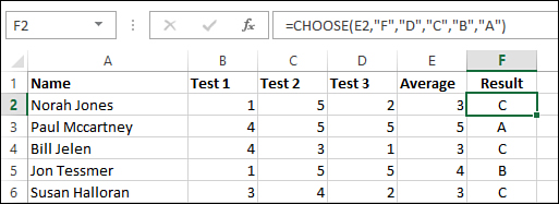
Figure 6.8. CHOOSE works for simple choices where you want to change a numerical value to something else, such as a text equivalent.

VLOOKUP

The VLOOKUP function matches your lookup value to a value in a table and returns data from a specified column in the matching row. This has many uses, such as returning customer information based on the customer ID or finding out if a value in list A is also in list B.

The syntax of the VLOOKUP function is as follows:

VLOOKUP(lookup_value, table_array, col_index_num, [range_lookup])

• lookup_value—The value to match in the leftmost column of the table_array.

• table_array—The entire range from which you want to look up and return a value.

• col_index_num—The column from the table_array from which to return the value. This is not equivalent to the column heading but instead is the location of the column in the table. For example, if the table begins in column G and the col_index_num is 2, a value from column H is returned.

• range_lookup—If TRUE or omitted, the table must be in ascending order by the first column for the function to match correctly. The function attempts to do an exact match. If this isn’t possible, it finds the first closest match from the top of the table, without exceeding the lookup value. If FALSE, the function only looks for an exact match. If not found, a #N/A error is returned.

Figure 6.9 shows how VLOOKUP can be used to return customer information to an invoice. The customer’s name is entered in cell B3. Functions in cells B4:B5 match the customer’s name in the table on the sheet Customer Data and return address and phone information. Note the use of IFERROR with VLOOKUP. If an exact match is not found, “Not Available” is entered in the cells, instead of the #N/A error.

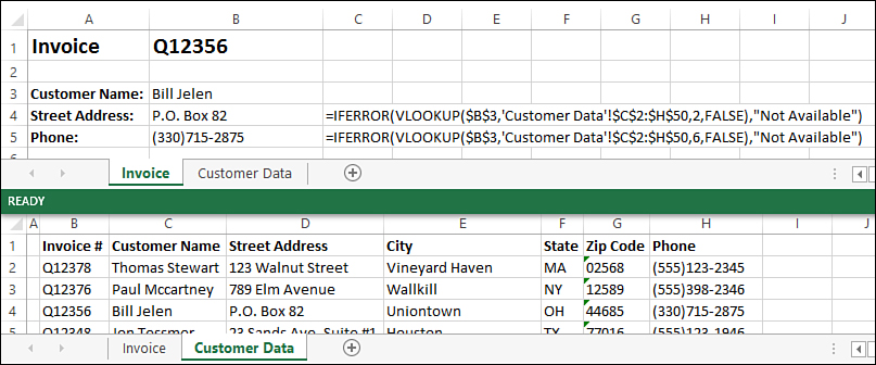
Figure 6.9. Use VLOOKUP formulas to return customer information from a table on another sheet.

VLOOKUP Troubleshooting

If VLOOKUP returns an error or incorrect value but you can manually verify that the lookup value is present in the table, the exact issue may be one of the following:

• If using FALSE for the range_lookup, the entire cell contents must match 100%. If you’re looking up “Bracelet” and the term in the table is “Bracelets,” Excel does not return a match.

• Be careful of extra spaces before and after a word. “Bracelet” and “Bracelet” are not matches—the first occurrence has a space at the end.

• If matching numbers, make sure both the lookup value and the matching value are formatted the same type—for example, both as General or one as General and the other as Currency, allowing Excel to still see them as numbers. Sometimes when importing data, numbers get formatted as Text. If you have a lookup value formatted as General and the matching value is formatted as Text, Excel does not see this as a match. See the section “When Cell Formatting Doesn’t Seem to Be Working Right” in Chapter 4, “Formatting Sheets and Cells,” for instructions on how to force the numbers stored as text to become true numbers.

• Make sure the table_array encompasses the entire table.

MATCH and INDEX

VLOOKUP works only when returning data from columns to the right of the lookup column. If your data is also to the left of the lookup column, use MATCH and INDEX together. For example, if you have a customer phone number, but not the name, and the table is set up like the one in Figure 6.9, you can use MATCH to return the row the phone number is in, then use that result in INDEX with the column you do want (column C).

The syntax of the MATCH function is as follows:

MATCH(lookup_value, lookup_array, [match_type])

The syntax of the INDEX function is as follows:

INDEX(array, row_num, [column_num])

The MATCH function looks up a value and returns its position (row or column) in an array:

• lookup_value—The value to match and return the location of

• lookup_array—The range from which to return the location

• match_type—A 1, 0, or -1 telling the function how to match the lookup_value

• If 1, the function returns the largest value that is less than or equal to the lookup_value. The lookup_array must be sorted in ascending order.

• If 0, the function returns the first value that is an exact match to the lookup_value.

• If -1, the function returns the smallest value that is greater than or equal to the lookup_value. The lookup_array must be sorted in descending order.

The INDEX function returns a value based on a row and column number:

• array—A range of cells from which to return a value

• row_num—The number of the row within the range to return a value from

• column_num—The number of the column within the range to return a value from

Figure 6.10 shows how the two functions are used to return information to the left of the customer name column. First, the MATCH function is used to locate which row in the customer list matches the name. That information is used in the INDEX function to tell it from which row to return the value.

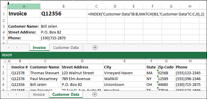
Figure 6.10. Use MATCH and INDEX to return information located to the left of the customer name.

OFFSET and MATCH

The INDEX function requires an array to be preselected to extract values from it. But if the size of the range increases and you don’t have a dynamic range formula setup, the function could fail. An alternative is the similar OFFSET function, which allows you to specify a cell a specific number of rows and columns from another cell.

The MATCH function is laid out in the previous section. The syntax of the OFFSET function is as follows:

OFFSET(reference, rows, cols, [height], [width])

• reference—The range from which you want to base the offset from.

• rows—The number of rows, either up (negative) or down (positive) you want to move from the reference.

• cols—The number of columns, either left (negative) or right (positive) you want to move from the reference.

• [height]—An optional value. It’s the number of rows by which you want to expand the selection. For example, if the reference is a single row and a height of 2 is used, then the selection will be two rows high.

• [width]—An optional value. It’s the number of columns by which you want to expand the selection. For example, if the reference is a single column and a width of 2 is used, then the selection will be two columns wide.

For example, you need to calculate the commission for your salespeople. You can place the sales values and commission rates in a table. Use a combination of the OFFSET and MATCH functions to look up and return the commission rate. The commission table may look like this:

9,999 or less: 1%

10,000 to 14,999: 1.2%

15,000 to 24,999: 1.3%

25,000 or higher: 1.5%

Create a table as shown at the top of Figure 6.11. Notice that the minimum and maximum sales values are placed in increasing order and that each value has its own column.

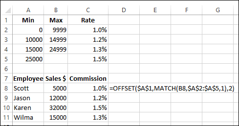
Figure 6.11. Instead of embedded IF statements, consider using a lookup table using lookup functions to return commission rates or other values based on comparisons.

The second table is the calculation table for the commission rate. First, MATCH is used to look up the Sales $ value in the above rate table. A match_type argument of 1 is used to return the row of the largest value that is less than or equal to the lookup value. With that information, we can now calculate the position of the correct rate. The reference is A1, the upper-left corner of the rate table. I could just as easily use C1, but for consistency in my formulas, I prefer to use the upper-left corner of the lookup table. Next is the MATCH function, returning the number of rows away from the reference and finally the number of columns away from the reference. All this together tells Excel exactly what cell and value I want returned.

INDIRECT

When you place a cell address in a formula, you aren’t just putting in some letters and numbers. That cell address has certain properties you can’t see or access, but Excel knows they are there. If you were to try to build a cell address by joining text, for example =”B” & “1”, all you would get in the cell is B1. But if you wrap that formula in INDIRECT, you turn that formula into a true cell address.

The INDIRECT function returns a reference specified by a string, allowing for dynamic cell references. Another way you can use INDIRECT is if you have sheet names that are also salespeople’s names; you can use INDIRECT to build a sheet name reference in a formula based on the salesperson’s name, as shown in Figure 6.12. You can change the name in the cell referenced by the function and instantly refer to another sheet.

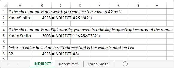
Figure 6.12. INDIRECT provides flexibility in creating dynamic cell references. There are a few rules to keep in mind if you’re going to use the function to create sheet name references.

The syntax of the INDIRECT function is as follows:

INDIRECT(ref_text, [a1])

• ref_text—Specifies a cell or string reference.

• a1—Specifies the type of reference in the cell ref-text. If TRUE or omitted, ref_text is treated as an A1-style reference. If FALSE, the ref-text is treated as an R1C1-style reference.

SUMIFS

SUMIFS allows you to sum a single column based on multiple criteria. For example, you can sum revenue between two dates or sum the quantity of a specific product in a specific region.

The syntax of the function is (optional arguments are in square brackets) as follows:

SUMIFS(sum_range, criteria_range1, criteria1, [criteria_range2, criteria2],...)

• sum_range—The range containing the cells to sum

• criteria_range1—The range of cells to evaluate for the first criteria

• criteria1—A number, expression, or text to match in criteria_range1

The sum_range and criteria_range must be the same number of rows. Key items to keep in mind when entering the criteria arguments in the function (cell references refer to Figure 6.13):

• An argument can be a direct cell reference, for example $H5 in the formula shown in cell I8.

• Words must be entered in quotation marks, for example “East” in the formula shown in cell I9.

• Equality and inequality symbols (<, >, >=, <=,=, <>) must be placed in quotation marks with the value in the comparison, as shown in cell I14.

• If using equality and inequality symbols with a cell reference, the cell reference should be outside the quotation marks around the symbol. Also, build the statement using the ampersand (&), as shown in cell I14.

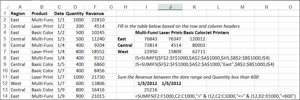
Figure 6.13. SUMIFS sums a column based on one or more criteria.

SUMPRODUCT

The SUMPRODUCT function multiplies corresponding components in argument arrays of the same size and returns the sum of the products. For example, if array1 is A1:A10 and array2 is B1:B10, the function is actually doing this: ((A1*B1)+(A2*B2)+(A3*B3)...(A10*B10)).

The syntax of the function is (optional arguments are in square brackets) as follows:

SUMPRODUCT(array1, [array2], [array3], ...)

SUMPRODUCT can also be used as a multiple criteria lookup, returning the sum of the values matching the criteria. This was a common use for the function before SUMIFS was introduced in Excel 2007 and is still useful if you’re sending a workbook to legacy Excel users.

The function can deal only with numbers. If the lookup values are strings, Excel has to be tricked into treating them like numbers. You can do this by placing a “--” (two unary minuses) in front of the comparison argument, like this: --(C1:C5=”Karen”).

When the function does the comparison (C1=Karen), it returns TRUE or FALSE. The first unary minus changes a TRUE to a -1 and a FALSE to -0 (there is no such thing as -0, so you would see 0 only if you looked into it). The second unary minus negates the first, changing TRUE to 1 and FALSE to 0. Now we have 1s and 0s, numbers that can be multiplied together with the value to sum.

Figure 6.14 shows a detailed breakdown of how the function works to do a sum with multiple criteria that include text values. Column A lists the number of printers and scanners sold by Karen and Joe. G1 uses SUMPRODUCT to calculate the number of printers sold by Karen.

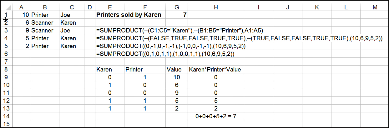
Figure 6.14. SUMPRODUCT can be used to do a multiple criteria lookup of text values.

Starting in E3, you can see the steps SUMPRODUCT takes to calculate the value. E3 shows the original formula in G1. E4 shows the first step into the calculation where Excel “opens” up the array and does the logic comparison (does C1 = Karen?) or lookup (A1=10, A2=6, etc.).

E5 uses the first unary minus to convert the TRUE and FALSE results to their numerical values of 0 and -1. E6 uses the second unary minus to convert any -1 values to 1.

The table starting at E8 shows the numerical values in a table layout so you can see the actual calculation. As you read across a row, multiply each value. For example, in row 9, it’s 0*1*10=0. Once each row value is calculated (column H), the values from each row are added together, as shown in H14, giving us the final result, 7.

Logical Functions

Logical functions allow decision making to be used on spreadsheets, either on their own, such as the IF function, or combined with other functions, such as the AND function.

The logical functions are (optional arguments are in square brackets) as follows:

• IF—Specifies a logical test to perform, returning one value if the formula evaluates to TRUE and another if it evaluates to FALSE. The function syntax is

IF(logical_test, [value_if_true], [value_if_false])

• IFERROR—Returns the value specified if the formula evaluates to an error; otherwise, returns the result of the formula. The function syntax is

IFERROR(value, value_if_error)

• AND—Returns TRUE if all its arguments are TRUE. Returns FALSE if any of the arguments evaluate to FALSE. The function syntax is

AND(logical1, [logical2], ...)

• OR—Returns TRUE if any of its arguments are TRUE. Returns FALSE if all the arguments evaluate to FALSE. The function syntax is

OR(logical1, [logical2, ...])

• NOT—Reverses the logic of its arguments. The function syntax is

NOT(logical)

• TRUE—Returns TRUE. TRUE can be entered directly into cells and formulas; it is provided as a function for compatibility with other spreadsheet applications.

• FALSE—Returns FALSE. FALSE can be entered directly into cells and formulas; it is provided as a function for compatibility with other spreadsheet applications.

IF/AND/OR/NOT

If you were to read an IF statement aloud, it would sound like this: “If this is true, then do this, else do this.” The first argument of an IF statement is a logic test usually using at least one of the comparison operators in Table 6.1. If the comparison resolves to TRUE, the second argument is returned to the cell. If the comparison resolves to FALSE, the third argument is returned.

Table 6.1. Comparison Operators

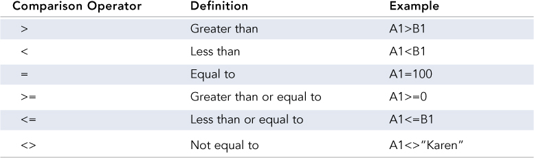
The second and third arguments can be numbers, text, formulas, or functions. If text, the words must be enclosed in quotations marks, unless returning TRUE or FALSE, because these are functions in their own right.

AND, OR, and NOT can be used to expand the first argument, allowing multiple comparisons or reversing a comparison. Figure 6.15 shows four examples of combining these functions to compare the data in columns A, B, and C in multiple ways. Below the title of each example is an example of the formula being used. All three calculated rows in each example use the same formula. The following sections review these examples.

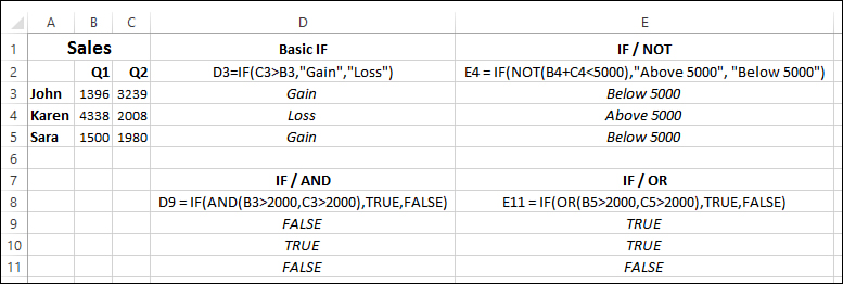
Figure 6.15. Use AND, OR, or NOT with IF statements to expand on the type of comparison the function can do.

Basic IF

Cells D1:D5 show an example of a basic IF statement “If the value under Q2 is greater than the value under Q1, then put Gain in the cell, else, put Loss.”

IF/NOT

Cells E1:E5 show an example of an IF statement using NOT to reverse the results of the logical test. The logical test is B4+C4<5000 and the result is FALSE (6346<5000). The use of NOT reverses the result, changing the FALSE to TRUE. So now, the IF statement would be read “If the sum of Q1 and Q2 is not less than 5000, then put Above 5000 in the cell, else, put Below 5000.”

IF/AND

Cells D7:D11 show an example of an IF statement using AND to do multiple logical tests. If both logical tests return TRUE, then the overall result is TRUE. But if just one of the tests returns FALSE, then the result is FALSE. The IF statement would be read “If Q1 and Q2 are both greater than 2000, then put TRUE in the cell, else, put FALSE.”

IF/OR

Cells E7:E11 show an example of an IF statement using OR to do multiple logical tests. If either of the logical tests returns TRUE, then the overall result is TRUE. The only way to have FALSE returned is if both logical tests return FALSE. The IF statement would be read “If either Q1 or Q2 is greater than 2000, then put TRUE in the cell, else, put FALSE.”

Nested IF Statements

A nested IF statement is when an IF statement is used as an argument within an IF statement, like this:

=IF(A1>B1, IF(B1>C1,0,IF(D1=C1,D1*B1,A1)),FALSE)

The above could be read “If A1 is greater than B1, then check if B1 is greater than C1. If it is, put 0 in the cell. Else, check if D1=C1 and if it is calculate D1*B1, else, put the value from A1 in the cell. But if A1 is not greater than B1, then put FALSE in the cell.” The second and third IF statements only get checked if the first IF statement is TRUE and the third statement only gets checked if the second one is FALSE.

Excel 2007, 2010, and 2013 allow 64 nested IF statements, but if you’re sharing the workbook with legacy Excel users, you’re limited to seven nested IF statements. Also, too many nested IF statements can be difficult to read, though you can use Alt+Enter to force line breaks in a formula. An alternative is to create a user-defined function using Select Case statements. For more information on this, refer to Chapter 15, “An Introduction to Using Macros and UDFs.”

Another alternative may be to rethink your formula and consider a different setup and function. Let’s say you need to calculate the commission for your salespeople. You may be tempted to do nested IF statements, but there are other solutions, some of which might be easier to read and update. Instead of putting all those values into the formula, place them in a table, and use a combination of the OFFSET and MATCH functions. See the section “OFFSET and MATCH” for a more detailed example.

IFERROR

If there’s a chance a formula may return an error, use the IFERROR function to prevent the error from appearing in the cell. Instead of an error, a text message or other value may appear.

In Figure 6.16, the top table uses a straightforward division formula (see formula in cell G5) to calculate the unit price. In cell F9, the column is summed, but returns an error because of the error in cell F5.

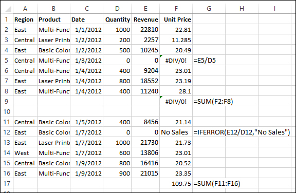
Figure 6.16. Use IFERROR to resolve potential problems in calculations before they arise.

The bottom table in Figure 6.16 uses IFERROR to return the text “No Sales” if an error occurs in the calculation, as shown in cell F12. In cell F17, the SUM function is used again, but this time there isn’t an error in the range to throw Excel off, and so the sum is calculated.

Date and Time Functions

Dates and times in Excel are not stored the same way we’re used to seeing them. For example, you may type 9/8/12 into a cell, but Excel actually sees 41160. That number, 41160, is called a date serial number. The formatted value, 9/8/12, is called a date value. Storing dates and times as serial numbers allows Excel to do date and time calculations.

Time serial numbers are stored as decimals, starting at 0.0 for 12:00 a.m. and ending at 0.999988425925926 for 11:59:59 p.m. The rest of the day’s decimal values are equivalent to their calculated percentage, based on the number of hours in a day, 24. For example, 1:00 a.m. is 1/24 or .04166. 6:00 p.m. would be the 18th hour of the day, 18/24 = 0.75.

Understanding how Excel stores dates and times is important so that you can successfully use formulas and functions when calculating with dates and times.

You might already be familiar with the functions that return the system date and time. DATE() returns the system date. NOW() returns the system date and time. The next few sections review additional functions in Excel for dealing with dates and times.

Functions to Convert and Break Down Dates

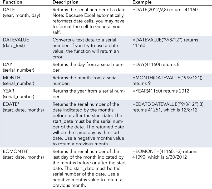
Table 6.2 lists the functions that can convert a date value to its serial value, or vice versa. It also lists the functions that can return part of a date, such as the month. The date used in the examples is September 8, 2012.

Table 6.2. Date Conversion Functions

Function to Convert and Break Down Times

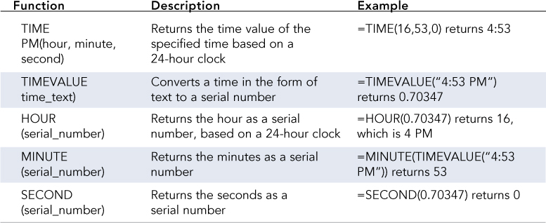
Table 6.3 lists the functions that can convert a time value to its serial value or vice versa. It also lists the functions that can return a part of a time, such as the hour. The time used in the examples is 4:53 p.m.

Table 6.3. Time Conversion Functions

Using Date Calculation Functions

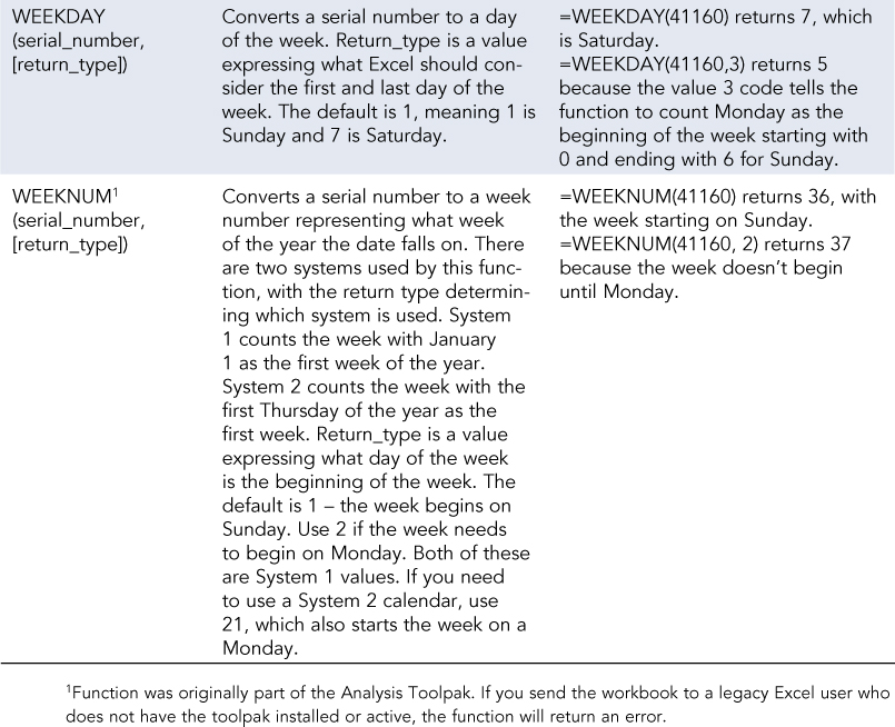
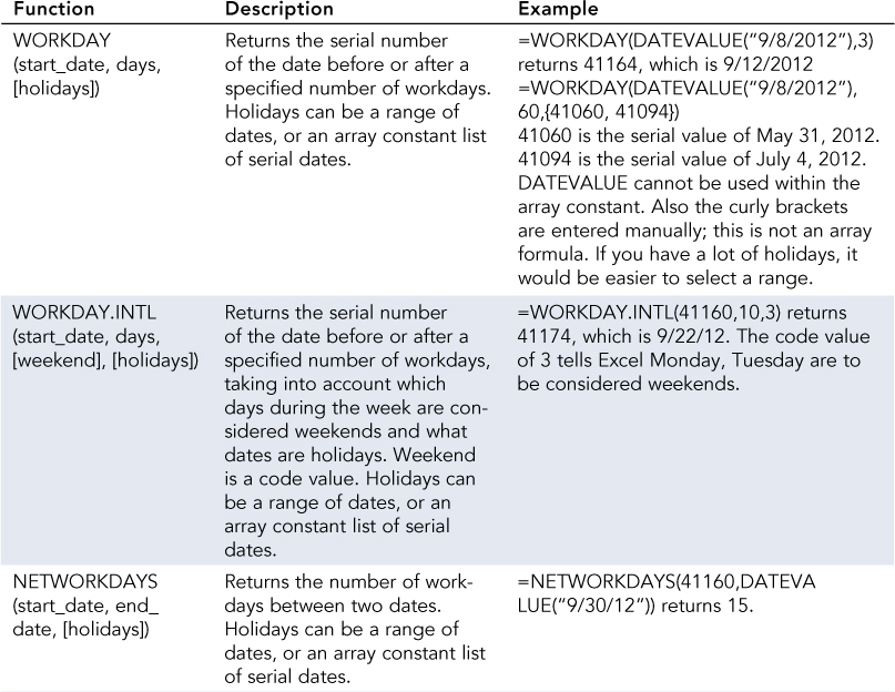
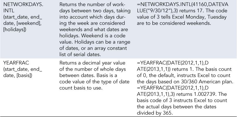
Table 6.4 lists functions that return calculated information, such as the end date based on a starting date, or the number of days between two dates. The date used in the examples is September 8, 2012. Square brackets denote optional arguments.

Table 6.4. Date Calculation Functions

Calculating Days Between Dates

If you need to find the number of days between two dates on a sheet, you can enter a direct formula, such as =F21-F20. After pressing Enter, you may get an odd answer, such as 1/25/1900. You didn’t have the formula cell formatted as date, but because the arguments are dates, Excel feels the answer should also be formatted as one. There’s nothing you can do about this—you will have to manually format the cell as General to get the actual number of days between the dates.

If you get a ###### error, the formula is trying to subtract a new date from an older date.

Calculating Overtime

You have a sheet similar to the one in Figure 6.17 where start and end times are entered; then the number of hours worked each day are calculated by subtracting the start time from the end time. At the end of the week, all the times are added together—and you get a number that is most definitely not correct, as shown in cell D7.

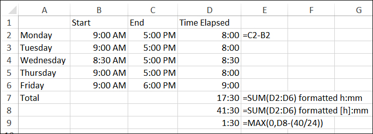
Figure 6.17. Use the proper time format to see the calculated time.

The problem isn’t the method of summing the column, but instead, the format applied to the cell. The standard format of h:mm can’t handle more than 24 hours. To get Excel to show more than 24 hours, change the format of the calculated cell to [h]:mm, as shown in cell D8.

If you have a sheet with daily work times, and you need to calculate the total number of hours worked and also the overtime, follow these steps:

1. For each workday, calculate the time elapsed, as shown in cell E2 of Figure 6.17.

2. Select the range of elapsed time.

3. Go to Home, Editing, and click the AutoSum button.

4. Right-click the cell containing the totaled time and select Format Cells.

5. On the Number tab, select the Custom category.

6. In the Type field, enter [h]:mm. Click OK to return to the sheet.

7. In the overtime cell, enter a MAX function that returns the greater of 0 or the calculated overtime. To calculate the overtime, divide the number at which overtime begins (example 40) by 24. Take that calculation and subtract it from the calculated time, as shown in cell D9.

8. Right-click the cell containing the overtime and select Format Cells.

9. On the Number tab, select the Custom category.

10. In the Type field, enter [h]:mm. Click OK to return to the sheet. This is a precaution in case the amount of overtime exceeds 24 hours.

Troubleshooting Dates and Times Stored as Strings

As long as the dates on a sheet are serial dates, you can perform a variety of calculations with them. If you receive a sheet where the dates are stored as strings (you may see ′4/19/12 in a cell and your formulas don’t work), there are two ways to convert the dates: either using Paste Special to add a blank cell onto the range or using text to columns to convert the column.

Using Paste Special to Convert Text to Dates and Times

To convert text dates to real dates using paste special, follow these steps:

1. Copy a blank cell.

2. Select the range of text dates to convert.

3. Go to Home, Clipboard, Paste, Paste Special, and select Add.

4. Click OK and the text dates will convert to dates that can be formatted and that Excel can do calculations with.

Using Text to Columns to Convert Text to Dates and Times

To convert a column of text dates to real dates using text to columns, follow these steps:

1. Select the range of text dates.

2. Go to Data, Data Tools, Text to Columns.

3. From the wizard dialog box that appears, make sure Delimited is selected and click Next.

4. In step 2, make sure the Space delimiter is not selected. Any other delimiter not being used in your cell can be selected. Click Next.

5. In step 3, select the Date option then the desired format.

6. Click Finish and the text dates/times will convert to dates/times that can be formatted and that Excel can do calculations with.

Goal Seek

Goal Seek, found under Data, Data Tools, What-If Analysis, adjusts the value of a cell to get a specific result from another cell. For example, if you have the price, term, and rate of a loan, you can use the PMT function to calculate the payment. But what if the calculated payment wasn’t satisfactory and you wanted to recalculate with additional prices? You could take the time to enter a variety of prices, recalculating the payment. Or use Goal Seek to tell Excel what you want the payment to be and let it calculate the price for you. A couple of things to keep in mind when using Goal Seek:

• You must have the formula in the Set Cell. Goal Seek works by plugging in values into your existing formula.

• A clear mathematical relationship between the starting and ending cells must exist.

Figure 6.18 calculates the monthly payment in cell B4 based on the price, term, and rate. I’ve decided I can make a larger monthly payment, but instead of entering prices, I’ll use Goal Seek to tell Excel my desired payment and have it figure out what value in the price cell will bring me closest to my payment. To do so, follow these steps:

1. Select cell B4, which is the cell whose value you want to be a specific value.

2. Go to Data, Data Tools, What-If Analysis, Goal Seek.

3. In the Set Cell field should be the address of the cell selected in step 1. If not, select the cell whose value you want sought.

4. In the To Value field, enter the value you want the Set Cell to be, such as 630.

5. In the By Changing Cell field, select the cell whose value you want Excel to change so the Set Cell field calculates to the desired value, in this case, cell B1.

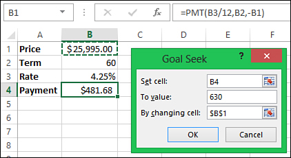
Figure 6.18. Use Goal Seek to find one value by changing one in another cell.

6. Click OK. Excel attempts to return a solution as close to the desired value as possible. If it succeeds, a message box appears showing the target value and the actual value it attained.

Using the Function Arguments Dialog Box to Troubleshoot Formulas

If you have one function using other functions as arguments and the formula returns an error, you can use the Function Arguments dialog box to track down which function is generating the error. To do this, place your cursor in the function name in the formula bar and click the fx button to the left of the formula. The dialog box opens, with the selected function filled in. You can review the arguments to make sure they are correct and falling into the correct fields. To check the next function, click the function name in the formula bar—you do not need to close the dialog box and start from the beginning.

Figure 6.19 shows a commission table returning incorrect values in the range C8:C11. The formula uses two functions, so it’s difficult to say exactly which one is the problem. To use the Function Arguments dialog box to inspect the formula and find the problem, follow these steps:

1. Select the cell with the formula to troubleshoot.

2. Place your cursor in the first function OFFSET in the formula bar.

3. Click the fx button to the left of the formula bar. The Function Arguments dialog box opens for the selected function, with its arguments filled in.

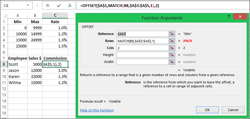
Figure 6.19. Use the Function Arguments dialog box to narrow down which function is causing a problem.

4. If you see the error in the selected function, you can fix it and click OK to recalculate the formula. Otherwise, continue to the next step.

5. In this case, the #N/A being returned for the Rows field shows that the error is somewhere in the MATCH function. It could be the MATCH function itself, or if that function used another function, you may have to dig deeper. To inspect another function, click it in the formula bar and it will load in the dialog box. In the case of the example, the Lookup_array of the MATCH function is not looking at all the data it needed to—the correct range is $A$2:$A$5.