4. Formatting Sheets and Cells

Now that you have your data on a sheet, you need to format it so that it’s easy to decipher and readers can quickly make sense of it. From simple font formatting, wrapping text, and merging cells to placing icons in cells so it’s obvious how one number compares with another, Excel has the tools you need to make reports visually interesting.

Adjusting Row Heights and Column Widths

If you can’t see all the data you enter in a cell or the data in a column doesn’t use up very much of the column width, you can adjust the column width as needed. Several methods are available for adjusting column widths on a sheet. Each method described here also works for adjusting row heights:

• Click and drag the border between the column headings—Place your cursor on the border between two column headings, as shown in Figure 4.1. Once the cursor turns into a two-headed arrow, you can click and drag to the right to make the column to the left wider or drag to the left to make the column narrower. The advantage of this method is you have full control of the width of the column. The disadvantage is that it affects only one column.

Figure 4.1. The border between columns is the key to quickly adjusting the column width.

• Double-click the border between the column headings—Excel automatically adjusts the left column to fit the widest value in that column. The advantage of this method is that the column is now wide enough to display all the contents. The disadvantage is if you have a cell with a very long entry, the new width may be impractical.

• Select multiple columns and drag the border for one column—The width of all the columns in the selection adjusts to the same width as the one you just adjusted.

• Select multiple columns and double-click the border for one column—Each column in the selection adjusts to accommodate its widest value.

• Apply one column’s width to other columns—If you have a column with a width you want other columns to have, you can copy that column and paste its width over the other columns by using the Column Widths option of the Paste Special dialog box.

• Use the controls on the ribbon—Select the column(s) to adjust. Go to Home, Cells, Format, Column Width. Enter a width and click OK.

• AutoFit a column to fit all the data below a title row—If you have a long title and need to fit the column to all the data below the title, double-clicking the border between column headings won’t work as this adjusts the column width based on the title. Instead, select the data in the column, without the title, and use the AutoFit Column Width option under Home, Cells, Format.

Using Font Size to Automatically Adjust the Row Height

The default row height is based on the largest font size in the row. For example, if cell F2 has a font size of 26, even if there is no other text in the row, the row automatically adjusts to approximately 33. You can take advantage of this to set the height of a row, instead of manually setting the row height. The advantage is that when a user tries autofitting the row height, your setting won’t change.

Changing the Font Settings of a Cell

Changing font aspects allows you to add emphasis to a selected range. There are multiple ways of accessing the font-changing tools in Excel. You can open the Format Cells dialog box by right-clicking a cell and selecting Format Cells, by pressing Ctrl+1 (the number one), or by going to Home, Cells, Format and from the drop-down, selecting Format Cells. The options are also available on the Mini toolbar in Excel, shown in Figure 4.2, and from the Font group on the Home tab.

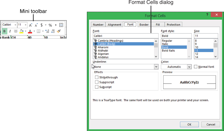
Figure 4.2. The Format Cells dialog box and the Mini toolbar, which appears above the context menu when you right-click over a cell, are just two ways you can change font settings.

Selecting a New Font Typeface

The default font in Excel is Calibri, but many others are available. To change the font, select the range, and then select a new font from the drop-down in the Font group, as shown in Figure 4.3. If your cell is viewable, you can preview the selection in the selected range as you move your cursor through the list.

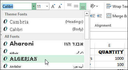
Figure 4.3. If your cell is viewable, you can preview the font selection in the selected range as you move your cursor through the list.

Increasing and Decreasing the Font Size

To change the font size, select the range, and then select a new size from the drop-down. The ribbon and Mini toolbar have two additional buttons next to the Font Size drop-down, shown in Figure 4.4. To increase the font size by one point (two after 12 point), click the A with the up arrow (A^); to decrease the font size by one point (two after 12 point), click the slightly smaller A with the down arrow (Av).

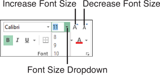
Figure 4.4. The Increase Font Size and Decrease Font Size buttons allow you to change the font size of the selected range with one click.

Applying Bold, Italic, and Underline to Text

The three icons for bold, italic, and underline toggle the property on and off. The Bold icon is a bold letter B. The Italic icon is an italic I. The Underline icon, which is a drop-down, is either an underlined U or a double-underlined D. To apply formatting, select the range and click the desired formatting button.

Applying Strikethrough, Superscript, and Subscript

The strikethrough, superscript, and subscript effects are available only in the Effects group on the Font tab of the Format Cells dialog box. To apply the formatting, select the cell or specific characters in the cell, right-click over the selection, and select Format Cells to bring up the dialog box and select the desired formatting option.

Changing the Font Color

In the ribbon and Mini toolbar, the Font Color drop-down is the button with the A underscored by a thick red line, which changes when you select a different color from the available colors. In the Format Cells dialog box, the Font Color drop-down is found on the Font tab. Any color in the drop-down can be applied to a cell.

Formatting a Character or Word in a Cell

All of the previous methods can also be applied to a single character or word in a cell, not just the entire cell contents. To change the formatting of just part of a cell, highlight the desired characters and use your preferred method of formatting.

Aligning Text in a Cell

The Alignment group on the Home tab consists of tools that affect how a value is situated in a cell or range. You can also access these controls from the Alignment tab of the Format Cells dialog box (refer to the beginning of the “Changing the Font Settings of a Cell” section for the various methods to open the dialog box).

There are six alignment buttons in the Alignment group, representing the most popular settings for how a value is situated in a cell. Top Align, Middle Align, and Bottom Align describe the vertical placement of the value in the cell. Align Text Left, Center, and Align Text Right describe the horizontal placement of the value in the cell. More options are available in the Format Cells dialog box on the Alignment tab. The Mini toolbar only has one button for horizontal alignment, which centers the text of the selected cell.

Merging Two or More Cells

Merging cells takes two or more adjacent cells and combines them to make one cell. For example, if you are designing a form with many data entry cells and need space for a large comment area, resizing the column might not be practical as it will also affect the size of the cells above it. Instead, select the range you want the comments to be entered in and merge the cells. Any text other than that found in the upper-left cell of the selection is deleted as the newly combined cell takes on the identity of this first cell.

On the Alignment tab in the Format Cells dialog box, there is a check box for Merge Cells. In the upper-right corner of the Mini toolbar is a toggle button (Merge/Unmerge) to merge and center the text of the selected range.

The Merge & Center drop-down in the Alignment group on the Home tab offers several options to merge cells in different ways:

• Merge & Center—This is the default action of the drop-down button. The selected cells will be merged and the text will be centered.

• Merge Across—If you have several rows where you want to merge the adjacent cells in the same row, you can select all the rows (and their adjacent columns to merge) and select Merge Across. See Figure 4.5.

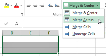
Figure 4.5. Notice that although several rows are selected, using Merge Across kept the separate rows intact.

• Merge Cells—Equivalent to the check box in the Format Cells dialog box, the selected range will be merged, retaining the alignment of the upper-left cell in the selection.

• Unmerge Cells—Use this option to unmerge the selected cells.

Use caution when merging cells because it can lead to potential issues:

• Users will be unable to sort if there are merged cells within the data.

• Users will be unable to cut and paste unless the same cells are merged in the pasted location.

• Column and row AutoFit won’t work.

• Lookup type formulas will return a match only for the first matching row or column.

Centering Text Across a Selection

As noted in the earlier section “Merging Two or More Cells,” merging cells can cause problems in Excel, limiting what you can do with a table. If you need to center text over several columns, instead of merging the cells, center the text across the multiple columns. To center a title across the top of a table without merging the cells, as shown in Figure 4.6, follow these steps:

1. Type your title in the leftmost cell to the table.

2. Select the title cell and extend the range to include all cells you want the title centered over.

3. Press Ctrl+1 or go to Home, Cells, Format, Format Cells to open the Format Cells dialog box.

4. Go to the Alignment tab.

5. From the Horizontal drop-down, select Center Across Selection.

6. Click OK.

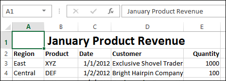
Figure 4.6. Use Center Across Selection instead of merging cells to center a title on a report.

Wrapping Text in a Cell to the Next Line

When you type a lot of text in a cell, it continues to extend to the right beyond the right border of the cell if there is nothing in the adjacent cell. You can widen the column to fit the text, but sometimes that may be impractical. If that’s the case, you can set the cell to wrap text, moving any text that extends past the edge of the column to a new line in the cell.

Normally, when you wrap a cell, the row height automatically adjusts to fit the text. If it doesn’t, make sure you don’t have the cell merged with another; Excel will not autofit merged cells. If there are merged cells, unmerge them and manually force an autofit (see the “Adjusting Row Heights and Column Widths” section). The row height will begin to automatically adjust again.

To turn on text wrapping, select the cell and go to Home, Alignment, Wrap Text or from the Format Cells dialog box, select Wrap Text on the Alignment tab. There is no option on the Mini toolbar.

Indenting Cell Contents

By default, text entered in a cell is flush with the left side of the cell, while numbers are flush to the right. To move a value away from the edge, you might be tempted to add spaces before or after the value. If you change your mind about this formatting at a later time, it can be quite tedious to remove the extraneous spaces.

Instead, use the Increase Indent and Decrease Indent buttons to move the value about two character lengths over. Increase Indent moves the value away from the edge it is aligned with. Decrease Indent moves the value back toward its edge.

When adjusting the Indent from the Format Cells dialog box, the Alignment tab uses a single Indent field with a number to indicate the number of indentations. The Mini toolbar does not offer options for indenting.

Changing the Way Text Is Oriented

Vertical text can be difficult to read, but sometimes limited space makes it a requirement. The Orientation button, which looks like ab written at a 45-degree angle, has five variations of Vertical Text, Angle Counterclockwise, Angle Clockwise, Vertical Text, Rotate Text Up, and Rotate Text Down. The Orientation section in Format Cells, Alignment offers more precise control (see Figure 4.7). There is no option on the Mini toolbar.

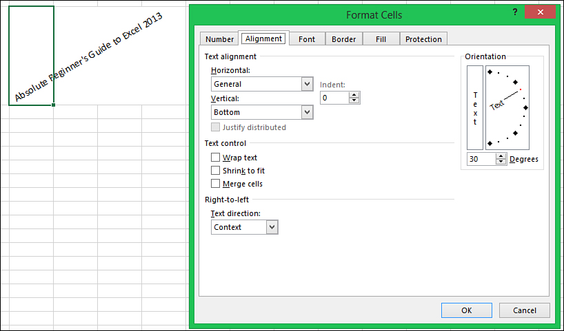
Figure 4.7. Use the Orientation settings to rotate the contents of a cell.

Reflowing Text in a Paragraph

There’s a very handy tool that’s not found with the other formatting tools. It is hidden in the Editing group on the Home tab. The button is the Fill button (a blue down arrow) and the option within it is Justify.

The Justify option reflows the text in a paragraph to fit a certain number of columns. For example, if you paste a paragraph directly into a cell with Wrap Text on, the height of the cell increases, but the column width is unaffected. Use Fill, Justify to reflow the text.

Be careful when selecting the range, because if you do not have enough empty rows available for the text to flow into, Excel will, after warning you, overwrite the rows below the selection.

To reflow text in a paragraph to fit a certain number of columns, follow these steps:

1. Ensure that the text is composed of one column of cells. The sentences can extend beyond one column, but the left column must contain text and the remaining columns must be blank.

2. Select a range as wide as the finished text should be. Ensure that the upper-left cell of the selection is the first line of text, as shown in Figure 4.8.

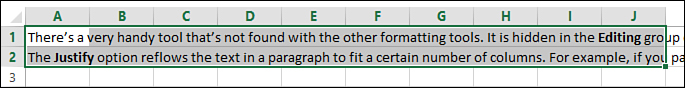
Figure 4.8. The number of columns selected determines the width of the final result.

3. From the Home tab, select Editing, Fill, Justify. You may receive a prompt that the text will reflow into more rows than selected. Click OK to continue. The text reflows so that each line is shorter than the selection range, as shown in Figure 4.9.

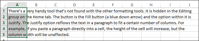
Figure 4.9. The text flows to the width of the original selection and down the number of rows it needs to.

Applying Number Formats with Format Cells

The way you see number data in Excel is controlled by the format applied to the cell. For example, you may see the date as August 21, 2012, but what is actually in the cell is 41142. Or you may see 10.5%, but the actual value in the cell is 0.105. This is important because when doing calculations, Excel doesn’t care what you see. It deals only with the actual values.

There are only a few formatting options on the Home tab in the Number group. This section reviews the formatting options available in the Format Cells, Number dialog box. To apply a number format, select the range, select the desired format from the dialog box, and click OK.

For a review of the Number Format drop-down and the Increase Decimal and Decrease Decimal buttons in the ribbon, see the “The Number Group on the Ribbon” section.

General

General is the default format used by all cells on a sheet when you first open a workbook. Decimal places and the negative symbol are shown if needed. Thousand separators are not.

Number

By default, the Number format uses two decimal places but does not use the thousands separator. You can change the number of decimal places, turn on the thousands separator, and choose how to format negative numbers, as shown in Figure 4.10.

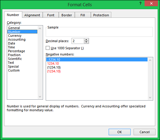
Figure 4.10. Additional options may be available when you select a format to apply.

Currency

The default Currency format displays the system’s currency symbol, two decimal places, and a thousands separator. You can change the number of decimal places, change the currency symbol, and select a format for negative numbers.

Accounting

Accounting is similar to Currency but automatically lines up the currency symbols on the left side of the cell and decimals points to the right side of the cell. The default Accounting format displays the system’s currency symbol, two decimal places, and a thousands separator. You can change the number of decimal places and the currency symbol.

Date

There is no default Date format. Sometimes Excel reformats the date you enter; sometimes it keeps it the way you entered it. You can select a date format from the list in the Type box, which also contains date and time formats.

The date formats vary from short dates, such as 4/5, to long dates, such as Monday, April 5, 2010. When selecting a date format, look at the sample above the Type list. It will help you differentiate between the format 14-Mar, which is March 14, and the format Mar-01, which is March 2001, not March 1.

Time

There is no default Time format. You can select a time format from the list in the Type box, which also contains two date and time formats.

Excel sees times on a 24-hour clock. That is, if you enter 1:30, Excel assumes you mean 1:30 a.m. But if you enter 13:30, Excel knows you mean 1:30 p.m.

If you need to display times beyond 24 hours, such as if you’re working on a timesheet adding up hours worked, use the time format 37:30:55, as shown in Figure 4.11.

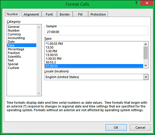
Figure 4.11. There are various time formats available.

Percentage

The default Percentage format includes two decimal places. When you apply this format, Excel takes the value in the cell, multiplies it by 100, and adds a % at the end. When you use the cell in a calculation, the actual (decimal) value is used. For example, if you have a cell showing 90% and multiply it by 1,000, the result will be (in General format) 900 (0.9*1,000).

If you include the % when you type the value in the cell, in the background Excel converts the value to its decimal equivalent, but the Percentage format is applied to the cell.

Fraction

The Fraction category rounds decimal numbers up to the nearest fraction. You can select to round the decimal to one, two, or three digits, or to round to the nearest half, quarter, eighth, sixteenth, tenth, or hundredth.

Scientific

The default Scientific category displays the value in scientific notation accurate to two decimal places. You can change the number of decimal places.

Text

There are no controls for the Text category. Setting this format to a cell forces Excel to treat the numbers in the cell as text, and you view exactly what is in the cell. If you set this format before typing in a number, the number becomes a number stored as text and may not work in some calculations.

Special

The Special category provides formats for numbers that do not fall in any of the preceding categories because the values are not actually numbers. That is, they aren’t used for any mathematical operations and instead are treated more like words.

The four special types are specific to U.S. formatting:

• ZIP Code—Ensures that East Coast cities do not lose the leading zeros in their ZIP Codes.

• ZIP Code + 4—Ensures that East Coast cities do not lose the leading zeros in their ZIP Codes and formats the +4 in ZIP codes.

• Phone Number—Formats a telephone number with parentheses around the area code and a dash after the exchange.

• Social Security Number—Uses hyphens to separate the digits into groups of three, two, and four numbers.

Creating a Custom Format

Despite all the options available in the preceding categories, not all the possible situations are covered. For example, you need to remove the - symbol from negative numbers and instead color the negative numbers red. Yet for calculation purposes, you still want the values to be negative. Or you need to add text, such as kg, to a cell without actually having the text in the cell, which would interfere with calculations. That’s why there’s the option of Custom formats, allowing you to create a format specific to your situation.

Custom formats are saved with the workbook they are created in.

Understanding the Four Sections of a Number Format

A custom format can contain up to four different formats, each separated by a semicolon.

You should keep several things in mind when creating a custom format:

• Use semicolons to separate the code sections.

• If there is only one format, it applies to all numbers.

• If there are two formats, the first section applies to positive and zero values. The second section applies to negative values.

• If there are three formats, the first section applies to positive values, the second section applies to negative values, and the third section applies to zero values.

• If all four sections are used, they apply to positive, negative, zero, and text values, respectively.

Figure 4.12 shows a custom number format using all four sections. The table in C9:D13 displays how the formats would be applied to different values. The M in in the first and second sections adds an M to the numerical values. The @ in the fourth section is a placeholder for any text the user types into the cell. Note the value in cell D11 is red, and a zero, not a blank, must be entered in cell C12 for “No Sales” to appear.

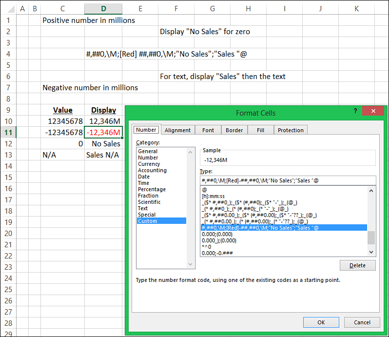
Figure 4.12. Use the four sections of a custom format to design formatting for positive, negative, zero, and text values.

Using Text and Spacing in a Custom Number Format

Excel can’t perform mathematical calculations on cells with text in them. For example, if you have a mileage chart and wanted to have “miles” in each cell, you wouldn’t be able to also sum those cells because the “miles” would throw Excel off. Instead of typing the text in the cells, you can apply a custom number format that would make it look like the word “miles” is in the cell. As shown in Figure 4.12, you can display both text and numbers in a cell using a custom format. To do this, enclose the text in double quotation marks. If you need only a single character, you can omit the quotation marks and precede the character with a backslash (). Some characters don’t need quotes or a backslash. These special characters are: $ - + / ( ) : ! ^ & ’ ~ { } = < > and the space character.

If you’re using the fourth section of the number format, include the @ sign where you want to display any text in the formatted cell. If the @ is omitted from the format, text entered in the cell will not be displayed.

To have Excel add space to a format, such as having Excel line up the decimals in a column on negative and positive numbers where the negative numbers are wrapped in parentheses, use an underscore followed by a character. In Figure 4.13, the format in column B doesn’t include the _) in the positive section of the format, and so the positive value in the cell is flush with the right margin. In contrast, the format in column C does include the _) and the decimal points beneath are lined up. It’s like having an invisible) in the cell.

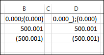
Figure 4.13. Use an underscore to instruct Excel to add a specific amount of space to a format.

To fill unused space in a cell with a repeating character, use an asterisk followed by the character to repeat. The repeating character can appear before or after the value in the cell. For example *-0 fills the leading space in the cell with dashes, whereas 0*^ fills in the trailing space with carets.

Using Decimals and the Thousands Separator in a Custom Number Format

Zeros are used as placeholders in a format when you need to force the place to be included, such as if you need to format all numbers with exactly three decimal places. If there aren’t enough digits to fill in the required decimal places, Excel adds zeros to the end of the value.

If you would like to display up to three decimal places, but it is not necessary, use the pound (#) sign as the placeholder. Excel shows a maximum of three decimal places, but if there are only two, it won’t fill in the third with a zero.

Use a question mark (?) on either side of a decimal to replace insignificant zeros if you will be using a fixed-width font (such as Courier) and want the decimal points to line up.

For example, to format the positive section to always show three decimal places and the negative section to show only what’s entered, use this custom format: 0.000;-0.###. Positive values will display exactly three decimal places, including a filler zero if needed, and negative values will display up to three decimal places, as shown in Figure 4.14.

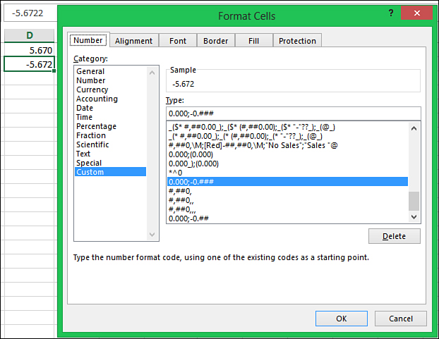
Figure 4.14. Create a custom format to treat positive and negative values differently.

To include a thousands separator, use a comma in the format, such as #,###.0. To scale a number by thousands, as shown in Figure 4.15, include a comma at the end of the numeric format for each multiple of 1,000.

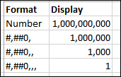
Figure 4.15. Use a comma as a thousands multiplier to change how a value is displayed.

Using Color and Conditions in a Custom Number Format

You can use eight text color codes in a format: red, blue, green, yellow, cyan, black, white, and magenta. You place the color in square brackets, such as [cyan]. It should be the first element of a numeric formatting section.

You can use conditions in conjunction with colors to create number formats that apply only when specific conditions are met. The colors and conditions can only be applied to the first two sections of the number format, but the other sections can still be used. For example, to color values greater than or equal to 50 in green, less than 50 in red, a blank for zeros, and have “Sales” joined to any existing text, use this format: [Green][>=50];[Red][<50];””;”Sales “@.

Using Symbols in a Custom Number Format

You can include various currency symbols, percent signs, and scientific notations in the number format.

If formatting with the exponent codes (E-,E+) and the format has a zero or pound sign (#) to the right of the code, Excel displays the number in scientific format and inserts an E or e. The number of zeros or pound signs to the right of the code determines the number of digits in the exponent. Code E+ places a minus sign by negative exponents and a plus sign by positive exponents. Code E- places a minus sign by negative exponents. Figure 4.16 shows the results of 0.00E+00 and 0.00E-00 on different numbers.

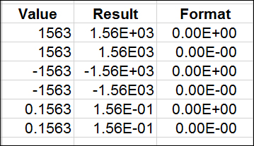
Figure 4.16. The use of E+ or E- makes a difference in how the scientific notation is formatted.

Formatting a Cell to Show the Cent (¢) Symbol

Normally when you apply a currency format, you get the dollar sign ($), but if the value is less than a dollar, you don’t get the cent symbol. To format a cell to show the cent symbol when the value is less than 1 and to show the dollar sign for values of 1 or greater, follow these steps:

1. Right-click over the cell to format and select Format Cells.

2. On the Number tab, select Custom from the Category list.

3. In the Type field, enter [<1]0.00¢;$0.00_¢ and click OK. To get the cent symbol, hold down the Alt key and type 0162 on the numeric keypad.

4. Values less than 1 will display with a ¢ at the end, such as 0.23¢. Values 1 or greater will display with the $ at the beginning, such as $12.23. A note of caution—negative values are technically less than zero and so a value such as -12.23 would format with the cent symbol (-12.23¢), but this format would work well on a sales column.

Using Dates and Times in a Custom Number Format

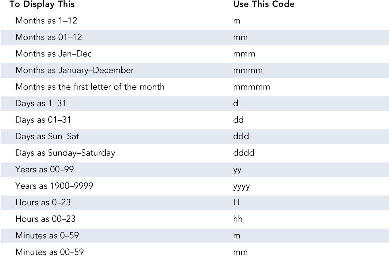
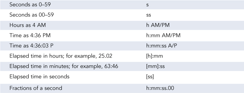
Date and Time formats have the greatest variety of codes available when it comes to creating number formats. Whereas there’s no real difference between the codes ## and ###, the difference between formatting a date cell mm or mmm are more obvious, as shown in Table 4.1.

Table 4.1. Date and Time Formats

There are a couple of things to keep in mind when creating date and time formats:

• If the time format has an AM or PM in it, Excel bases the time on a 12-hour clock. Otherwise, Excel uses a 24-hour clock. See the previous section “Time” for more information on entering times in Excel.

• When creating a time format, the minutes code (m or mm) must appear immediately after the hour code (h or hh) or immediately before the seconds code (ss) or Excel displays months instead of minutes.

When Cell Formatting Doesn’t Seem to Be Working Right

Most of the time, you can type in a number and then set the formatting, and the cell will reflect the formatting. This works about 99% of the time. But there is that 1% of cases that can cause a headache until you understand what is going on.

You’ve spent hours designing your sheet, copying ranges from various workbooks, and moving data around. You have a column of numbers and add a SUM function at the bottom. A few things may happen:

• The data sums, but the number doesn’t look correct.

• After pressing Enter, you see the formula exactly as you typed it in. It doesn’t sum the selected range.

• You see #### in a cell.

Check the format of the cell in question. If you were using the cell for something else earlier, it might still retain that format, such as text. If you’re looking at the formula cell, change the format to General. You still see the formula. That’s because the format has been applied to the cell, but not the contents of the cell. You need to force the format by entering the cell (F2, or double-click) and then pressing Enter.

If the issue is the range being summed, you can either go to each cell and force the formatting onto the contents as described previously, or refer to the section “Fixing Numbers Stored as Text” in Chapter 3, “Getting Data onto a Sheet.”

If you see ### in a cell, try increasing the size of the column. Sometimes Excel doesn’t automatically adjust the column width for an entered number.

The Number Group on the Ribbon

The Number group on the Home tab has several quick formatting options. The Number Format drop-down in the Number group of the Home tab has 11 formatting options available. Figure 4.17 shows an example of each format.

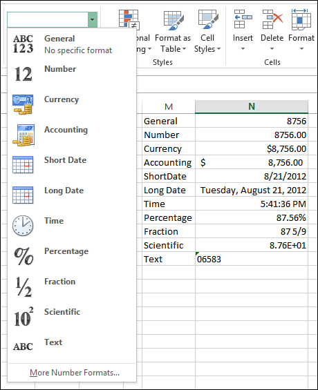
Figure 4.17. The Number Format drop-down offers many quick formatting options.

Below the Number Format drop-down is a drop-down button with a dollar sign ($) on it, the Accounting Number format. This button applies the accounting format to the selected range. From the drop-down, you can select different currency symbols.

Also beneath the drop-down are buttons for applying the Percent Style (%) and Comma Style (,) formats to a selection.

Use the Increase Decimal and Decrease Decimal buttons on the Home tab in the Number group (see Figure 4.18) to quickly increase and decrease the number of decimal places shown in number formats that use decimals. The Increase Decimal button has an arrow pointing left, whereas the Decrease Decimal button has an arrow pointing right.

Figure 4.18. The Number Format drop-down offers many quick formatting options.

Adding a Border Around a Range

The Borders drop-down in the Font group on the Home tab includes 13 of the most popular border options. These borders are applied to the selected cell or range, either the inside borders or the outside borders, depending on your selection. For more options, go to the Borders tab in the Format Cells dialog box.

When applying a border, Excel sees the entire selection as one object and applies the border you select to the selection, not the individual cells that make it up. For example, if you select a range consisting of five rows and apply the Bottom Border, the border appears only in the last cell, not at the bottom of each cell in the selection.

Formatting a Table with a Thick Outer Border and Thin Inner Lines

You can apply multiple border formats on top of each other. For example, if you want your table to have a Thick Box Border with thin inner lines, that option doesn’t existing in the drop-down. Instead, you have to apply the following steps to create a table that has a thick outer border and a thin border around each inner cell, as shown in Figure 4.19:

Figure 4.19. You can apply multiple selections from the Borders drop-down to a selected range to get the desired design.

1. Select the range to format.

2. From the Borders drop-down, select the All Borders option.

3. Return to the Borders drop-down and select the Thick Box Border option.

Coloring the Inside of a Cell

Fill Color refers to the color applied inside of a cell; it is represented by a paint bucket on its button in the Font group of the Home tab and on the Mini toolbar. When you click the button, a drop-down of available colors opens up. As you move your cursor over the colors, the selected range automatically updates to reflect the color your cursor is currently over. When you’ve decided on the color you want, click the color; the drop-down closes and the range is colored as specified.

The Format Cells, Fill tab dialog box offers additional Fill Effects, such as patterns, styles, and gradient fills. Pattern Color and Pattern Style work together to fill a cell with a pattern (various dots, lines) in the selected color. This effect is placed on top of the Background color. A gradient fill is when a color slowly changes from one color to another within a cell.

Applying a Two-Color Gradient to a Cell

Instead of filling a cell with a single solid color, you can apply a two-color gradient to a range by following these steps:

1. Select one or more cells. If you select a range, the gradient will repeat across the range.

2. Press Ctrl+1 to open the Format Cells dialog box.

3. Go to the Fill tab.

4. Click the Fill Effects button. The Fill Effects dialog box, shown in Figure 4.20, opens.

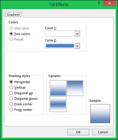
Figure 4.20. The Fill Effects dialog box offers more options for applying color inside of a cell.

5. Select a color from the Color 1 drop-down.

6. Select a different color from the Color 2 drop-down.

7. Select a shading style from the Shading Styles section.

8. Make a selection from the Variants section. The Sample box updates to reflect your selection.

9. Click OK twice.

Creating Hyperlinks

Hyperlinks allow you to open web pages in your browser, create emails, and jump to a specific cell on a specific sheet in a specific workbook. For web and email addresses, Excel automatically recognizes what you’ve typed in and applies the format accordingly, turning the cell into a clickable link.

If you want to link to a sheet, you have to go through the Insert Hyperlink dialog box, shown in Figure 4.21. You can open the dialog box by right-clicking on a cell and selecting Hyperlink or clicking Insert, Links, Hyperlink.

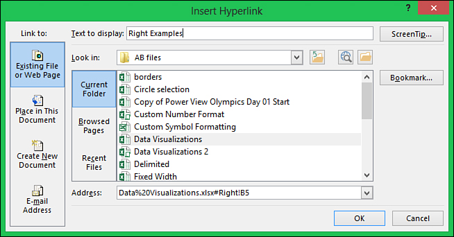
Figure 4.21. Use hyperlinks to help users quickly jump to sheets and specific ranges.

Creating a Hyperlink to Another Sheet

Being able to create a hyperlink to a sheet can be useful if you want to create a table of contents for a large workbook or a series of workbooks.

If you select just a sheet, Excel defaults to cell A1 on the sheet, but you can link to any specified cell. To create a hyperlink to a specific sheet, follow these steps:

1. Select the cell where you want the link.

2. Go to Insert, Links, Hyperlink and the Hyperlinks dialog box opens.

3. Browse to the workbook you want to link to. If you want to link to a cell in the current workbook, click the Place in This Document button.

4. If linking to an external workbook, click the Bookmark button to open the Select Place in Document dialog box. If linking to the active workbook, continue to step 5.

5. Select the sheet from the Cell Reference list. If you have a specific cell address you want the link to go to, enter it in the Type the Cell Reference field. Or, if you have a name assigned to the cell, select it from the Defined Names list. In that case, you don’t have to enter a cell reference.

6. Click OK.

7. If the cell selected in step 1 is blank, the Text to Display field at the top of the dialog box shows the destination for the hyperlink. You can type in new text if desired.

8. Click OK. The next time you click on the cell, you will follow the link.

Quick Formatting with the Format Painter

The Format Painter is a handy, but tricky, little icon in the Clipboard group on the Home tab. It’s handy because it enables you to quickly copy the formatting of one cell to another. It’s tricky because whether you single-click or double-click the button affects how it functions. If you click the button once, you can copy the format of the selected range to one other range. If you double-click the button, it remains on, enabling you to copy from the format of the selected range to as many other ranges as needed. Use the Esc key, or click or double-click the button again to turn it off.

To copy a format from a source range to a single destination range, follow these steps:

1. Select the source range.

2. Click the Format Painter button once. The cursor changes to a paintbrush with a plus sign, as shown in Figure 4.22.

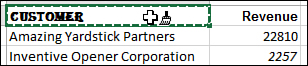
Figure 4.22. When the Format Painter is activated, the cursor changes to include a paintbrush.

3. Select the cell in the upper-left corner of the destination range if the range is the same size. If the destination range is larger, select the entire range.

4. The operation is complete and the cursor changes back to normal. If you accidentally selected the wrong range, undo and start over.

Dynamic Cell Formatting with Conditional Formatting

An unformatted sheet of just numbers isn’t going to grab your audience’s attention. But you don’t have time to create a colorful report—or do you? Conditional formatting allows you to quickly apply color and icons to data. The quick formatting options consist of the following:

• Data Bars—A data bar is a gradient or solid fill of color that starts at the left edge of the cell. The length of the bar represents the value in the cell compared with other values in the range the format is applied to. The smallest numbers have just a tiny amount of color, and the largest numbers in the range fill the cell.

• Color Scales—A color scale is a color that fills the entire cell. Two or three different colors are used to relay the relative size of each cell to other cells in the range the format is applied to.

• Icon Sets—An icon set is a group of three to five images that provide a graphic representation of how the number in a cell compares with the other cells in the range the format is applied to.

The quickest way to apply one of the conditional formats is to select all the cells you want to apply it to, go to Home, Conditional Formatting, click the formatting type, and select one of the formatting options from the submenu that appears, as shown in Figure 4.23. As you move your cursor over the options, your range changes to reflect the connection. When you find the formatting you want, click it, and it will be applied to your range.

Figure 4.23. Quickly apply formatting to your data by selecting one of the prebuilt options in the Conditional Formatting drop-down.

Applying Multiple Icon Sets

You can mix and match the individual icons. To use a green check mark for values in the top 67%, a red stoplight for items below 33%, and a yellow exclamation point for everything in between, follow these steps:

1. Select the range to which you want to apply the formatting.

2. On the Home tab, go to Conditional Formatting, Icon Sets, More Rules.

3. Click the first drop-down under the Icon heading and select the green check mark, as shown in Figure 4.24.

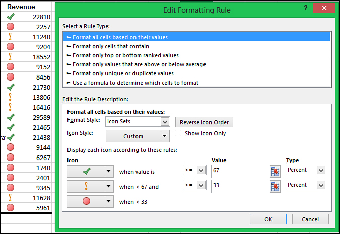
Figure 4.24. You can mix and match the conditional formatting icons.

4. To the right of the drop-down, select >= from the drop-down.

5. Enter 67 in the Value field.

6. Select Percent from the Type drop-down.

7. Click the second drop-down under the Icon heading and select the yellow exclamation point.

8. To the right of the drop-down, select >= from the drop-down.

9. Enter 33 in the Value field.

10. Select Percent from the Type drop-down.

11. Click the third drop-down under the Icon heading and select the red stoplight.

12. Click OK.

Conditional Formatting Using the Built-in Rules

Use the preset conditional formats if all you need is to format all the cells in a range based on how they compare with each other. But if your needs are more advanced, such as formatting only the top 10% or only cells that meet a specific condition, then you need to apply formatting using rules.

Under Conditional Formatting, Highlight Cells Rules and Top/Bottom Rules options, you’ll find several built-in rules that you can apply to your data. Apply selected formatting to the following:

• Cells containing values greater than, less than, between, or equal to the value you specify

• Cells containing specific text

• Cells containing a date from the last day, two days, and so on

• Cells containing duplicate values

• Cells containing the top or bottom n items

• Cells containing the top or bottom n%

• Cells containing values above or below the average

Mixing Cell Formats with the Built-in Rules

For all of the preceding built-in rules, you can apply one of Excel’s preset formats or design your own custom format. To apply a custom format to the top n items in the selected range, follow these steps:

1. Select the range to which you want to apply the formatting.

2. On the Home tab, go to Conditional Formatting, Top/Bottom Rules, Top 10 Items.

3. Enter the number of items you want formatted.

4. From the Format drop-down, select Custom Format.

5. From the Format Cells dialog box that opens, design the format you want applied (see Figure 4.25). You can go to any of the tabs (Number, Font, Border, and Fill) to make your selections. The only change you cannot make is to the font type and size on the Font tab.

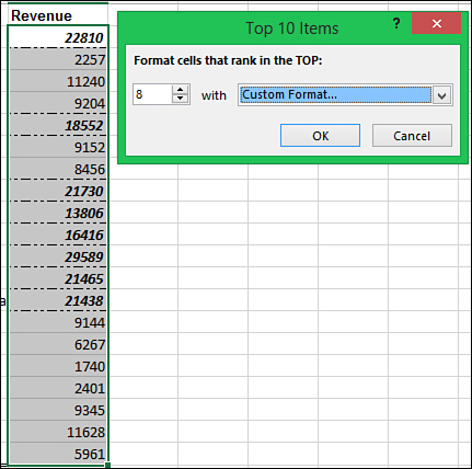
Figure 4.25. The Custom Format option of the Top 10 Items dialog box allowed me to apply a bold italic font and a border around the top 8 items in the range.

Building Custom Conditional Formatting Rules

You can customize any of the prebuilt rules, but if what you need is not listed, you’ll want to build your own conditional formatting rule based on a formula. For example, you’ve set up a data validation drop-down in one section of a sheet, and based on the selection, you want to highlight certain rows in a table in another section. A built-in formula won’t do this for you. You’ll need to apply a formula to the table that looks at the value in the drop-down then applies conditional formatting.

The formula box, shown in Figure 4.26 has a few rules for writing a formula:

• The formula must start with an equal (=) sign.

• The formula must evaluate to a logical value of TRUE or FALSE or the equivalents of 1 and 0.

• If you use your mouse to select cells on the sheet, Excel inserts the address using absolute referencing. If relative referencing is what you need, press the F4 key three times to toggle away the dollar signs in the formula.

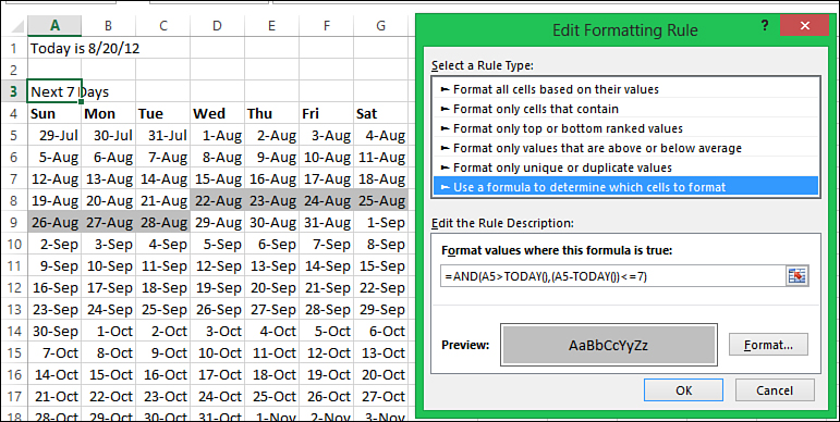
Figure 4.26. Use a custom formula to highlight the next seven days in your calendar.

For more information on absolute versus relative referencing, see the section “Relative Versus Absolute Formulas” in Chapter 5, “Using Formulas.”

• The formula you write will apply to the topmost left cell of your selection, so you need to look at the Name box in the formula bar and see what cell is the active cell. If you are writing a relative formula, write the formula as it would appear for the active cell. Excel will apply the formula appropriately to all the other cells you have selected. In Figure 4.26, the first cell in the range the formatting is applied to is cell A5 (29-Jul), which is also referenced in the formula.

• By default, the keyboard navigation keys (up arrow, down arrow, left arrow, right arrow, Page Up, Page Down, Home) are tied to the sheet and won’t work in the Formula field. If you try to use the arrow keys to change your cursor position while typing in the Formula field, Excel will instead place the cell address you just selected. To work around this behavior, press F2 before using the navigation keys. You can verify what mode you are in by looking in the lower-left corner of the status bar. There are three modes:

• Enter—The default mode for entering a formula in the Formula field. Using the navigation keys changes the selection on the sheet.

• Edit—The mode for using the navigation fields to move through the Formula field.

• Point—The mode for selecting cells on the sheet. Excel automatically switches to this mode when selecting cells on the sheet.

To set up a conditional format based on a formula, select the range it applies to and, from the Home tab, go to Conditional Formatting, New Rule, and select Use a Formula to Determine Which Cells to Format from the Select a Rule Type box. Enter your logical formula in the Formula field and set the desired Format.

Combining Conditional Formatting Rules

You can have multiple conditions evaluate to True and as each condition is met, the format is applied to the cell. For example, one rule sets the fill color to gray and another rule italicizes the contents, as shown in Figure 4.27. If both rules are met, the cell is formatted in italic with a gray fill. If a cell meets one condition, only the corresponding format is applied. If the formatting of the rules is conflicting, for example the first rule applies a red font and the second rule applies a blue font, the formatting of the first rule, the red font, is applied.

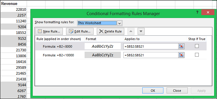
Figure 4.27. Setting up multiple rules can apply multiple formatting to cells.

Stopping Further Rules from Being Processed

Because rules are applied starting at the top, you might want to prevent further rules from being applied if a certain condition is met. In that case, check the Stop If True option in the Conditional Formatting Rules Manager for the rule you want to be the last if the condition is true. For example, in Figure 4.28, values below 8,000 were italic with a gray fill. But if you want to differentiate between items below 8,000 and those between 8,001 and 10,000 (without setting up a rule referencing the specific range), you would check the Stop If True for the first rule, as shown in Figure 4.28.

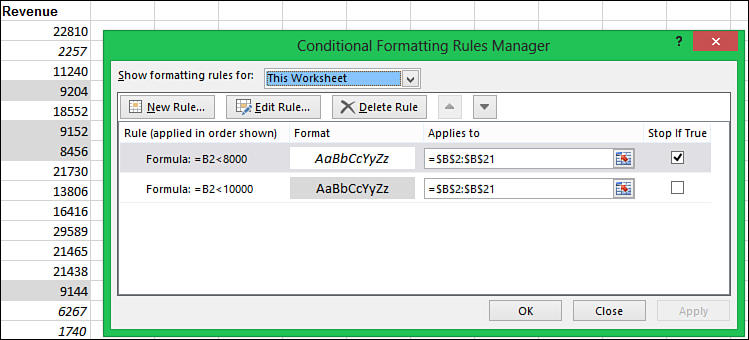
Figure 4.28. Check the Stop If True check box to prevent further rules from being applied to the data.

Clearing Conditional Formatting

You can set more than one conditional formatting rule on a range, so if you want to replace a format with another, you need to clear the previous rule. Or, you might want to clear all the formatting on a sheet. To clear conditional formatting, go to Home, Conditional Formatting, Clear Rules. From the drop-down that appears, you can select from the following options:

• Clear Rules from Selected Cell

• Clear Rules from Entire Sheet

• Clear Rules from This Table

• Clear Rules from This PivotTable

You can also select Clear Format from the Quick Analysis tool, which appears in the lower-right corner of a multiple cell selection.

Editing Conditional Formatting

Whether you’ve applied one of Excel’s quick apply formats or created your own, there might come a time when you need to edit the conditional formatting, whether it be the formatting you applied or the range you applied it to.

To edit conditional formatting, select Manage Rules from the Conditional Formatting drop-down. From the Show Formatting Rules For drop-down at the top, select which formatting rules you want to view. You can then select the rule and click Edit Rule.

Using Cell Styles to Quickly Apply Formatting

You’re probably used to using styles in Word but never realized that styles are also available in Excel. Select a range in Excel and go to Home, Styles, Cell Styles. Move your cursor over the predefined styles and watch your range update to reflect the styles.

You aren’t limited to these predefined styles. You can create and save your own style for use throughout the workbook it’s saved in. To quickly create a custom style in the active workbook, follow these steps:

1. Select a cell with all the formatting styles needed.

2. Go to Home, Styles, Cell Styles, New Cell Style.

3. If there is any type of formatting you do not want as part of the style, such as the alignment, unselect that style option.

4. Enter a name for the style in the Style Name field and click OK.

Using Themes to Ensure Uniformity in Design

Themes are collections of fonts, colors, and graphic effects that can be applied to a workbook. This can be useful if you have a series of company reports that need to have the same color and fonts. Only one theme can affect a workbook at a time.

Excel includes several built-in themes, which you can access from the Themes drop-down under Page Layout, Themes. You can also create and share themes you design.

A theme has the following components, which you can apply individually, instead of applying an entire Theme package:

• Fonts—A theme includes a font for headings and a font for body text.

• Colors—There are 12 colors in a theme: 4 for text, 6 for accents, and 2 for hyperlinks.

• Graphic effects—Graphic effects include lines, fills, bevels, shadows, and so on.

Applying a New Theme

The Themes group on the Page Layout tab has four buttons:

• Themes—Allows you to switch themes or save a new one

• Colors—Allows you to select a new color palette from the available built-in themes

• Fonts—Allows you to select a new font palette from the available built-in themes

• Effects—Allows you to select a new effect from the available built-in themes

Before applying a theme, arrange the sheet so you can see any themed elements such as charts or SmartArt. Then go to Page Layout, Themes and watch the elements update as you move your cursor over the various themes in the Themes drop-down. When you find the one you like, click it, and it will be applied to the workbook.

If you just want to change a theme component, make a selection from the component’s drop-down in the same way you would a theme.

Creating a New Theme

To create a new theme, you need to specify the colors and fonts and select an effect from the respective component’s drop-down. Then, under the Themes drop-down, choose Save Current Theme to save the theme.

To create a new theme, follow these steps:

1. Select Page Layout, Themes, Colors, Customize Colors.

2. To change an item’s color, such as Accent 5 in Figure 4.29, choose its drop-down to open the color chooser.

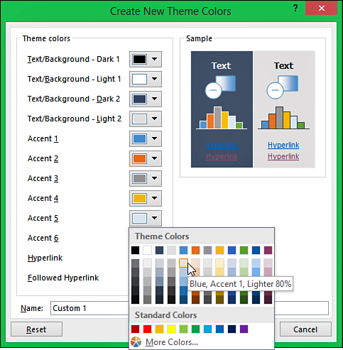
Figure 4.29. You can customize different aspects of a theme. As you select an item and change the color, the Samples on the right side of the dialog box will update.

3. When you find the desired color, click it to apply it to your theme.

4. Repeat steps 2 and 3 for each color you want to change.

5. In the Name field at the bottom, type a name for your color theme.

6. Click Save.

7. Select Page Layout, Themes, Fonts, Customize Fonts.

8. To change the Heading font, choose its drop-down to open the list of available fonts.

9. When you find the desired font, click it to apply it to your theme. The Sample box on the right updates to reflect your selection, as shown in Figure 4.30.

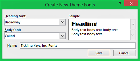
Figure 4.30. Create a custom theme using your organization’s specific font type.

10. Repeat steps 8 and 9 for the Body font.

11. In the Name field at the bottom, type a name for your font theme.

12. Click Save.

13. Select Page Layout, Themes, Effects.

14. Select an effect from the gallery of built-in effects, shown in Figure 4.31.

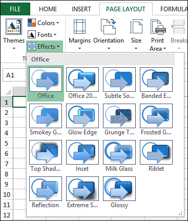
Figure 4.31. Select an Effect theme to change the default design of objects you insert, such as shapes.

15. Go to Page Layout, Themes, Save Current Theme.

16. Browse to where you want to save the theme, type a name for it, and click Save.

Sharing a Theme

To share a theme with other people, you must send them the *.thmx file you saved when you created the theme.

When they receive the file, they should save it to either their equivalent theme folder or some other location and use the Browse for Themes option under Page Layout, Themes, Browse for Themes.