3. Getting Data onto a Sheet

Data entry is one of the most important functions in Excel—and one of the most tedious, especially when the data is repetitive. This chapter shows you tricks for copying down data, fixing entered data, and helping your users enter data correctly by providing a predefined list of entries.

Types of Data You Enter into Excel

It’s important to differentiate types of data because Excel treats each differently. You tell Excel what kind of data is in a cell by how you type it into the cell or by how you format the cell. Data in Excel can fall into one of four categories.

• Numbers—Numeric data that can be used for calculation purposes.

• Text—Alphabetic or numeric data that is not used for calculation purposes. Examples of numeric text are phone numbers or Social Security numbers.

• Dates and Times—Although dates and times may be considered alphanumeric, there are occasions where you might want to perform calculations on the values, so it is important to identify the data correctly to Excel.

• Formulas and Functions—It’s important that Excel knows you’re entering a formula or it will treat what you enter like text. This topic is covered in detail in Chapter 5, “Using Formulas.”

You can’t combine types of data in a cell. You can type “5 oranges,” but Excel will see that as text. It won’t separate the “5” as a number and the “oranges” as text. If you want to deal with the 5 as a number, then you need to enter it into its own cell.

Entering Different Types of Data into a Cell

How you intially type data into a cell affects how Excel interprets it. You can save yourself some time if you let Excel format your data, but it will only do so properly if it can understand what you want. The following sections will help you help Excel understand what you want.

Typing Numbers into a Cell

Numbers are the simplest thing to type into a cell. You select a cell, type in a number, press Enter or Tab, and you’re done.

Typing Text into a Cell

If you simply select a cell and start typing without any forethought, you might get unexpected results. For example, select a cell and type the ZIP Code for Chester, MA, which is 01011, and press Enter or Tab. The beginning 0 disappears and all you see is 1011, as shown in Figure 3.1.

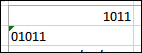
Figure 3.1. Excel tries its best to decipher the data you enter, but sometimes you have to help it out.

The reason this happens is because Excel assumes you are typing in a number, and numbers do not start with zeros. Although ZIP Codes are numeric, they aren’t numbers—that is, you don’t do any math with them. You need to plan ahead—know that you are entering numeric data that should be treated like text, and you need to let Excel know this. To let Excel know that you are entering a number that should be treated like text, type an apostrophe before you type the number.

Select another cell and this time type ′01011 and then press Enter or Tab. You’ll notice that the beginning zero remains. But you don’t see the starting apostrophe. Also, the ZIP Code is aligned to the left side of the cell instead of the right. This is another default action Excel takes when you enter data—it aligns the values for numbers, dates, and times to the right and text to the left.

When you type alphabetic characters into a cell, you don’t need to worry about a leading apostrophe. Nor do you need to worry about the apostrophe if you are mixing numbers and letters in the cell. But if you do have an apostrophe because it’s habit, that’s OK because Excel ignores leading apostrophes. However, if you need an apostrophe at the beginning of a cell, then enter two apostrophes—only the second one will show.

Typing Dates and Times into a Cell

Dates and times are another category in which it’s important for Excel to know what you are typing in. But in this case, the important thing to remember is to not put an apostrophe or other character before your date or time. Excel is very smart about date and time entry, and if you simply type it in, it does a very good job of deciphering your data.

Excel uses the system-configured date format. For example, in the United States, when entering numeric dates, the month comes first. For example, May 14, 2012 is written as 5/14/12.

If you enter only a month and day, Excel will append the current year. But this also means that if you enter a fraction that could be interpreted as a date, such as 3/4, Excel will convert it to a date, 3/4/12. To enter a fraction, you must format the cell as Fraction before entering it.

Dates must always include a day, month, and year, even if not all three will appear when the cell is formatted (see Chapter 4, “Formatting Sheets and Cells,” for more details on how formatting affects what you see but not actually what’s in the cell).

When entering times, you must enter it using a 24-hour clock, also known as military time or include the a.m. or p.m.

When entering a date, the time is included. But you might not see the part you didn’t type in until the cell is formatted to show it.

Controlling the Next Cell Selection

If you’re typing a single column list into Excel, you might get frustrated as the next selection moves to the next cell to the right when you want it to go down to the next cell. Or if your list has multiple columns, you find the next cell selection going down instead of to the right. You don’t have to put up with how Excel moves to the next cell selection. You can use several tricks to control what cell you enter data into next.

Entering Data in a Multicolumn List

Normally, when you press the Enter key as you enter data, the active cell moves directly down the column. If instead you want the selection to move to the right, you use the Tab key.

You can take advantage of these default actions to enter data in a multicolumn list, having Excel smoothly move from column to column to the next row. To make this happen, you must use the Tab key to move from one column to the next. When you get to the end of your data entry row, press Enter. Excel keeps track of which column you started your data entry on and returns you there, making it easier to start the next row of data.

Changing the Next Cell Direction when Pressing Enter

If you don’t want to use both Tab and Enter, you can go to File, Options, Advanced, After Pressing Enter, Move Selection, and change the Direction from Down to Right. But Excel will no longer move the selection to the next row when you get to the last column as explained in the previous section—because it doesn’t realize you are at the last column.

Preselecting the Data Range

If you have the selection set to move right when you press Enter, you can tell Excel when to go down to the next row by selecting the range into which you are entering data before you begin the data entry. In this way, Excel knows when you’ve reached the last column and will move down to the next row.

Using a Named Range to Indicate Data Entry Cells

If the data you need to fill in isn’t in consecutive columns or rows, such as the form shown in Figure 3.2, you can configure Excel to jump around to the different cells as you press the Enter key. You do this by setting up the data entry cells in a named range.

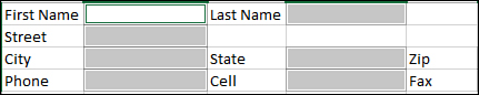
Figure 3.2. You can jump quickly from one highlighted cell to the next by setting those cells to be a named range.

To set up a named range to assist in data entry, follow these steps:

1. Ignore the first data entry field, and select the second field.

2. Hold down the Ctrl key and select each data entry field in the order you want to enter the data.

3. After all the other data entry fields have been selected, while still holding down the Ctrl key, select the first field.

4. Type a name for the selected range in the Name box and press Enter.

5. The next time you need to enter data in the fields, select the named range from the Name box drop-down and the fields will be highlighted, as shown in Figure 3.2. Begin entering data in the first field and press Tab or Enter to automatically go to the next field, repeating until you are done.

Using Copy, Cut, Paste, Paste Special to Enter Data

You can copy or cut data from different sources, such as other workbooks, Word documents, or web pages, and paste the information onto a sheet. Depending on how the data appeared in the original source, you might have to modify it after you paste it in Excel.

One of the ways you can clean up data copied or cut from another source is to use the Paste Special command instead of just Paste. To access this special command, go to Home, Clipboard and click the arrow on the Paste button or right-click on a cell. Various Paste Special options will appear. If you place your cursor over one of the icons, a tip appears, as shown in Figure 3.3. You can access more options by clicking Paste Special at the bottom of the drop-down.

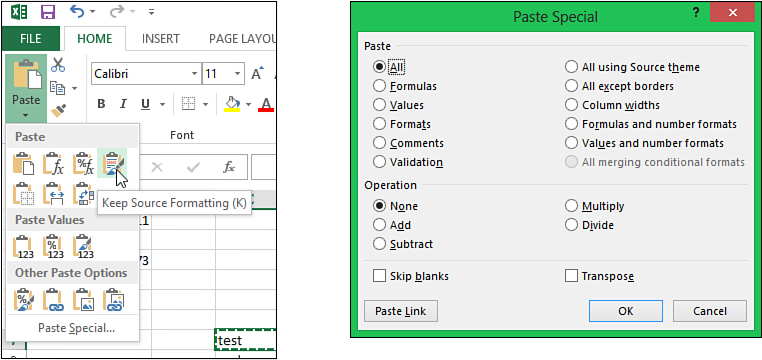
Figure 3.3. The Paste Special drop-down provides quick access to the more commonly used options. Click Paste Special at the bottom of the list to access the full dialog box.

Using Paste Special with Ranges

Figure 3.3 shows the Paste Special options available if pasting a range copied or cut from within Excel. The Paste area of the dialog box has different paste options you can choose from. For example, if you select Values, you will only paste the value of what you copied. The formatting and formulas will not be pasted. If you do want the original formatting but also the values, select Values and Number Formats. If you want a combination of values and comments, then you need to use Paste Special twice, selecting Values once and then Comments the second time.

The Operation area allows you to perform simple math on the selected range. For example, if you have a list of prices that need to go up by 1.5%, type .015 in a cell and copy the cell. Select your range of prices and bring up the Paste Special dialog box. From the dialog box, select Values (so you don’t lose any formatting you have on your prices) from the Paste area and Multiply from the Operation area. Click OK. Your prices will have increased by 1.5%.

Using Paste Special with Text

If you copy or cut data within a cell (versus the entire cell) or from a non-Excel source, such as a Word document or web page, the Paste Special options are limited. Depending on the source, text, or graphic, you may get the options shown in Figure 3.4.

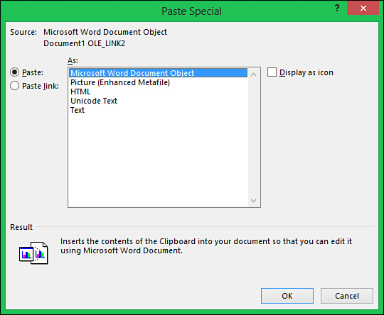
Figure 3.4. When doing a Paste Special with text, there are fewer options available.

As you select an option in the As list box, an explanation appears in the Result area at the bottom of the dialog box. If you select the Paste Link option to the left of the list, you’ll also be able to link the pasted data to its original source.

If available, the Display as Icon option lets you paste an icon instead of the text. Double-clicking on the icon opens the text in an editing application (for example, if pasting text from a Word document, you can edit the text in Word).

Using Paste Special with Images and Charts

When pasting images and charts, the dialog box is similar to that shown in Figure 3.4, but the As list box options differ, listing various image types. The different types can affect image resolution and workbook size.

Using Paste to Merge a Noncontiguous Selection in a Row or Column

If you try to copy/paste a noncontiguous selection from different rows and columns, an error message appears. But if the selection is in the same row or column, Excel allows you to copy and paste the data. When the data is pasted, though, it is no longer separated by other cells, as shown in Figure 3.5. You can use this method to create a table of specific values copied from another table.

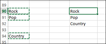
Figure 3.5. Data from rows 90, 91, and 94 was copied from the table on the left to create the list on the right using the method explained in this section.

Using Text to Columns to Separate Data in a Single Column

Data, Data Tools, Text to Columns can be used to separate data in a single column into multiple columns, such as if you have full names in one column and need a column with first names and a column with last names. When you select the command, a wizard dialog box opens to help you through the process. In step 1 of the wizard, select whether the text is Delimited or Fixed Width (see the next sections for definitions of Delimited and Fixed Width). In step 2, you provide more details on how you want the text separated. In step 3, you tell Excel the basic formatting to apply to each column.

If you have data in the columns to the right of the column you are separating, Excel overwrites the data. Be sure to insert enough blank columns to not overwrite your existing data before beginning Text to Columns. See the section “Inserting an Entire Row & Column” in chapter 2, “Working with Workbooks, Sheets, Rows, Columns, and Cells,” for instructions on how to insert columns.

Working with Delimited Text

Delimited text is text that has some character, such as a comma, tab, or space, separating each group of words that you want placed into its own column. To separate delimited text into multiple columns, follow these steps:

1. Highlight the range of text to be separated.

2. Go to Data, Data Tools, Text to Columns. The Convert Text to Columns Wizard opens.

3. Select Delimited from step 1 of the wizard, as shown in Figure 3.6, and click Next.

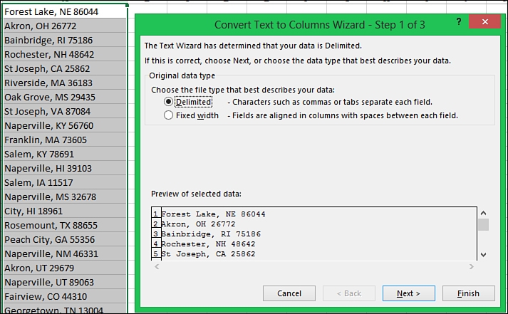
Figure 3.6. Select the Delimited option to separate text joined by delimiters, such as commas, spaces, or tabs.

4. Select one or more delimiters used by the grouped text, as in Figure 3.7, and click Next.

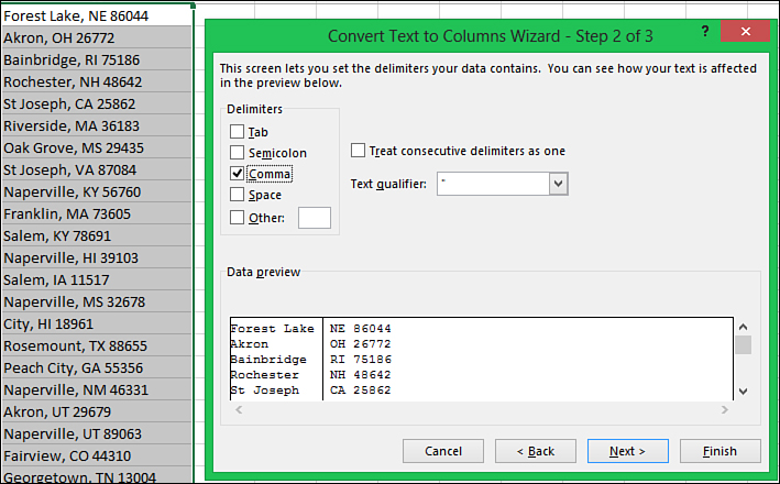
Figure 3.7. Select the Delimited option to use the comma as a delimiter between the city, state, and ZIP Code.

If you need more than one delimiter but one of the delimiters is used normally in the text, such as the space between city names and the space between a state and ZIP Code (Sioux Falls, SD 57057), consider running Text to Columns twice: once to separate the city (Sioux Falls) from the state ZIP Code (SD 57057) and again to separate the state and ZIP Code.

5. For each column of data, select the data format. For example, if you have a column of ZIP Codes, you need to set the format as Text so any leading zeros are not lost. But be warned—setting a column to Text prevents Excel from properly identifying formulas entered into that column.

6. Click Finish. The text is separated, as shown in Figure 3.8.

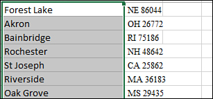
Figure 3.8. Using Text to Columns with a comma delimiter separated the city from the state and ZIP Code. Run the wizard again on the state ZIP Code column with a space as a delimiter to split up that data.

Working with Fixed-Width Text

Fixed-width text describes text where each group is a set number of characters. You can draw a line down all the records to separate all the groups, as shown in Figure 3.9. If your text doesn’t look like it’s fixed width, try changing the font to a fixed-width font, such as Courier. It’s possible that it’s fixed-width text in disguise.

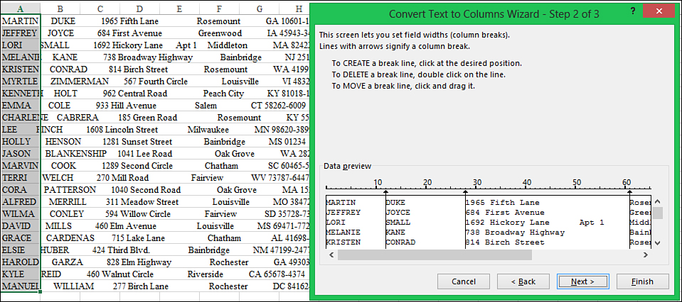
Figure 3.9. Use the Fixed Width option when each group in the data has a fixed number of characters.

To separate fixed-width text into multiple columns, follow these steps:

1. Highlight the range of cells that includes text to be separated.

2. Go to Data, Text to Columns.

3. Select Fixed Width from step 1 of the wizard and click Next.

4. Excel will guess at where the column breaks should go, as shown in Figure 3.9. You can move a break by clicking and dragging it to where you want it, insert a new break by clicking where it should be, or remove a break by double-clicking it. Click Next.

Don’t worry about leading spaces—Excel will remove them for you.

5. For each column of data, select the data format. For example, if you have a column of ZIP Codes, you need to set the format as Text so any leading zeros are not lost, as shown in Figure 3.10. But be warned—setting a column to Text prevents Excel from properly identifying formulas entered into that column.

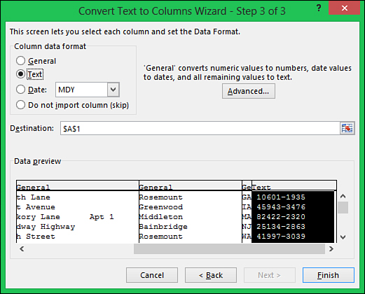
Figure 3.10. In step 3 of the wizard, set the format of each column. If you have numeric text, such as ZIP Codes, make sure you configure the wizard to treat the column as text so you don’t lose any leading zeros.

6. Click Finish.

Inserting Symbols and Equations into a Cell

Sometimes you need more than the symbols available on the keyboard, such as a copyright or registered trademark symbol. Some people have the Alt+number combination memorized, but if you’re like me, you don’t. No worries, though—if you go to the Insert tab, the Symbols group has commands for inserting equations and symbols.

First, select the cell where you want the symbol to appear. Next, select the Symbol option, and a window appears where you can search for the symbol you want. Once you find it, double-click on it, or click on it once and then click the Insert button. The symbol appears in the cell. The dialog box remains open in case you want to enter more symbols.

An equation isn’t the same as a formula. The formulas entered in Excel are meant to do calculations on the sheet. An equation doesn’t perform a calculation. Instead, it shows how a calculation is performed, using variables instead of numbers, like E=mc². If you click on the down arrow of the Equation button, a list of popular equations appears. If you don’t see the one you want, click the Equation button itself. A frame with Type Equation Here will appear on your sheet. Also, two new ribbons will appear—Drawing Tools and Equation Tools. Use the commands on the Equation Tools, Design tab to create your equation. Use the commands on the Drawing Tools, Format tab to format the frame in which the equation appears. When you’re done with the equation, just click elsewhere on the sheet.

Using Web Queries to Get Data onto a Sheet

A web query allows you to link a range to text from a web page. As the web page updates, the data on the sheet also updates. To retrieve data from a web page, follow these steps:

1. Go to Data, Get External Data, From Web. The New Web Query dialog box opens.

2. From the Address field at the top, navigate to the desired web page and it will load. If Excel is able to retrieve data from the web page, a yellow box with a black arrow appears near the data.

3. Place your cursor over the box and a frame appears around the data that box is tied to. Not all areas of a web page are retrievable. If you find a box that has the data you want, click the box and it turns into a green box with a black check mark.

4. Select as many sections as you need, then click the Import button at the bottom of the dialog box.

5. From the Import Data dialog box, select the cell where you want the data to appear. If you don’t like the current cell address shown, you can click on the sheet and the dialog box updates with a new sheet address. Click OK.

6. After a few seconds, depending on your Internet connection, the data appears on the sheet.

By default, the data refreshes every 60 minutes. You can refresh manually by clicking Data, Connections, and from the Refresh All drop-down, select Refresh. Or you can configure the automatic refresh time by going to Data, Connections, Properties or right-clicking the data and selecting Data Range Properties. Either way opens the External Data Range Properties dialog box where you can set the refresh time by selecting Refresh Every x Minutes and changing the value in the field, as shown in Figure 3.11.

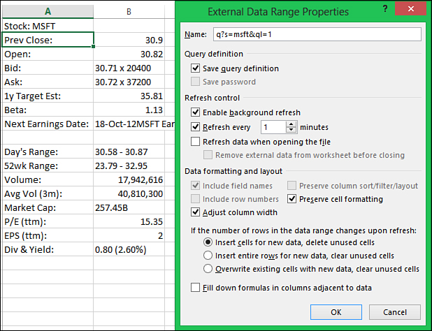
Figure 3.11. Use a web query to return an automatically updating summary of stock information for MSFT.

Using Series to Quickly Fill a Range

The fill handle, shown in Figure 3.12, can speed up data entry by completing a series for you. Excel comes with several preconfigured series, such as months, days of the week, and quarters. You can also add your own series, as described in the “Creating Your Own Series” section later in this chapter.

Figure 3.12. Use the fill handle to quickly fill in a series.

Extending a Series Containing Text

To extend a series containing text, enter the text you want the series to start with and press Ctrl+Enter to exit the cell, but keep it selected. Place your cursor over the lower-right corner of the cell until a black cross appears. Click the mouse button and as you hold it down, drag the fill handle.

You don’t need to start at the beginning of the series. You can start anywhere in the series and Excel will continue it, starting over if you drag the handle long enough. For example, if you begin a series in A1 with Sunday and drag the fill handle to A8, Sunday will appear again, repeating the series.

Extending a Numerical Series

If you try to fill numerical series based off of a single cell entry, Excel just copies the value instead of filling the series. There are four ways to get around this:

• Enter at least the first two values of the series before dragging the fill handle.

• Hold down the Ctrl key while dragging the fill handle.

• If there is a blank column to the left or right of the numerical column, include that column in your selection when dragging the fill handle down. For example, if you enter 1 in A1 then select A1:B1 (B1 is blank); when you drag the fill handle down, the series in column A is filled down.

• Hold the right mouse button down while dragging the fill handle and select Fill Series from the context menu that appears when you release the mouse button.

Creating Your Own Series

You can teach Excel the lists that are important to you so that you can take advantage of the series capabilities in Excel. You can take almost any list of items on a sheet and create a custom list for use in filling or sorting.

To create a custom list, follow these steps:

1. Create your list on the sheet and select the range.

2. Go to File, Options, Advanced, General, Edit Custom Lists.

3. The range you selected is already in the Import List from Cells field at the bottom of the Custom Lists dialog box, so click Import.

4. The list is added to both the Custom Lists and List Entries list boxes, as shown in Figure 3.13. The next time you type an item from your list and drag the fill handle, Excel fills in the rest of the series for you.

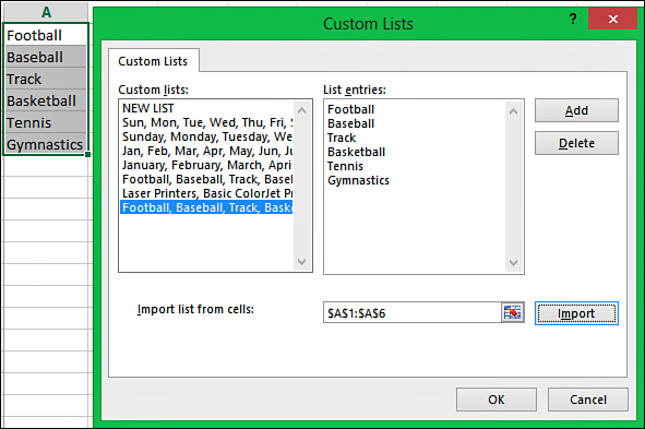
Figure 3.13. Create a custom list for use in filling in a series.

Editing Data

Now that you know how to enter data into a blank cell—how do you edit data already in a cell? If you select a cell and start typing, you’ll overwrite what was originally in the cell. You have three methods to choose from:

• Double-click—When you place your cursor over a cell and it’s a big white cross, double-click and the cursor appears wherever you double-clicked at, so you can go directly to a word or between numbers.

• Formula bar—Select the cell and then click where you want to edit in the formula bar.

• F2—Select the cell and press F2. The cursor appears at the right end of data in the cell.

When you’re done making changes, press Enter or whatever method you prefer to exit out of the cell and save your changes. If you change your mind about the changes while you’re still in the cell, press Esc and you’ll exit the cell without saving your changes.

Editing Multiple Sheets at One Time

You can change the exact same range on multiple sheets at the same time by grouping the sheets and making the change to one of the sheets. For example, you can enter the word Sales in cell A1 of all the selected sheets. Or you can apply a bold format to cell C2 in a group of sheets.

To make a change to multiple sheets by just changing one sheet, follow these steps:

1. Go to one of the sheets you need to change.

2. While holding down the Ctrl key, select the tabs of the other sheets you want to make the same change to. This groups the sheets together.

3. Make the changes to the active sheet.

4. To ungroup the sheets, select another sheet, or right-click on a sheet tab and select Ungroup Sheets.

Clearing the Contents of a Cell

To clear the data from a range, leaving the cells otherwise intact, such as the formatting, select the range and press the Delete key or right-click over the selection and choose Clear Contents.

Clearing an Entire Sheet

To clear a sheet of all data, but leave any formatting intact, click the intersection between the headers, shown in Figure 3.14, and press Delete or right-click and choose Clear Contents.

To clear a sheet of all data and formatting, select the entire sheet using the intersection between the headers, right-click and select Delete, or go to Home, Cells, Delete.

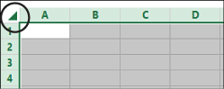
Figure 3.14. Clicking the intersection of the row and column headers selects all the cells on the sheet.

Working with Tables

When you enter information in multiple columns on a sheet, it is often referred to as a table, as in a table of data. But Excel also has a special term for a setting you can apply to a data table, imbuing it with special abilities and rules. This term is also Table. When your data table is defined as a Table, additional functionality in Excel is made available. For example, with Excel’s intelligent Tables, the following additional functionality becomes available:

• AutoFilter drop-downs, shown in Figure 3.16, are automatically added to the headings.

• You can apply predesigned formats, such as banded rows or borders.

• You can remove duplicates based on the values in one or more columns.

• You can toggle the total row on and off.

• Adding new rows or columns automatically extends the table.

• You can take advantage of automatically created range names.

Defining a Table

For your data to convert to a Table, it must be set up properly. This means that, except for the headings row (row 1 in Figure 3.15), each row must be one complete record of the data set—for example, a customer or inventory item—as shown in Figure 3.15. Column headers are not required, but if they are included, they must be at the top of the data. If your data does not include headers, Excel inserts some for you.

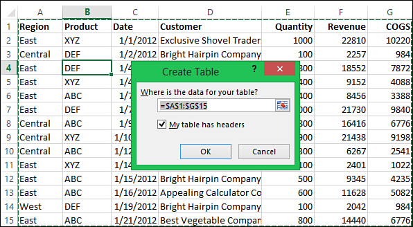
Figure 3.15. Set up your data properly to define it as a Table. Make sure the Create Table dialog box includes your entire data set and properly reflects the existence of headers.

After your data is set up properly, you can define the Table with one of the following methods. Select a cell in the data set and then do the following:

1. Go to Insert, Tables, Table.

2. Go to Home, Styles, Format as Table, and select a style to apply to the data.

3. Press Ctrl+T.

4. Press Ctrl+L.

When you use any one of the preceding methods, Excel determines the range of your data by looking for a completely empty row and column. The Create Table dialog box opens, showing the range Excel has defined. You can accept this range or modify it as needed. To modify it, you can click on the sheet and, holding down the mouse button, drag to create a box enveloping your entire data set. You can also modify it by editing the cell addresses in the Create Table dialog box.

If Excel was able to identify headers, the My Table Has Headers dialog box will be selected, so make sure that Excel has correctly identified whether your data has headers and click OK. If there were no headers, make sure the box is unselected and click OK. Your table will be formatted with AutoFilter drop-downs in the headers, as shown in Figure 3.16.

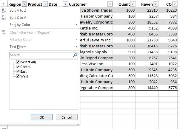
Figure 3.16. A Table automatically has AutoFilter drop-downs in the headers.

Expanding a Table

After your data is defined as a Table, the Table automatically expands as you add adjacent rows and columns. If you don’t want the new entry to be part of the Table, you can tell Excel by clicking the lightning bolt icon that appears and then selecting either Undo Table AutoExpansion or Stop Automatically Expanding Tables, as shown in Figure 3.17.

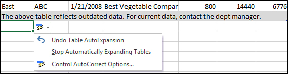
Figure 3.17. If you don’t want a new row or column to be part of the Table, instruct Excel to undo or stop the autoexpansion.

To manually resize a Table, click and drag the angle bracket icon in the lower-right corner of the Table. You can also select a cell in the Table and go to Table Tools, Design, Properties, Resize Table. Specify the new range in the Resize Table dialog box that opens.

Adding a Total Row to a Table

When you go to Table Tools, Design, Table Style Options, Total Row, Excel adds a total row to the bottom of the active Table. By default, Excel adds the word Total to the first column of the Table and sums the data in the rightmost column, as shown in Figure 3.18. If the rightmost column contains text, Excel returns a count instead of a sum.

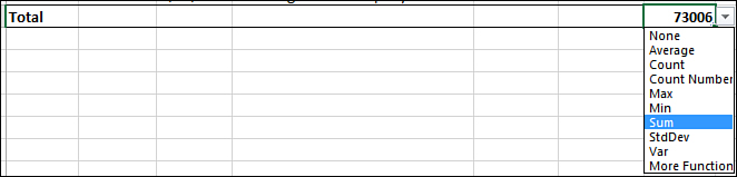
Figure 3.18. Selecting the Total Row check box adds a total row to the bottom of the Table. Use the drop-downs in each cell in this row to add or change the function used to total the data in the above column.

Each cell in the total row has a drop-down of functions that can be used to calculate the data above it. For example, instead of the sum, you can calculate the average, max, min, and more. Just make a selection from the drop-down and Excel inserts the formula in the cell.

Fixing Numbers Stored as Text

Sometimes when you import data or receive data from another source, the numbers might be converted to text. When you try to sum them, nothing works. That is because Excel will not sum numbers stored as text.

When numbers in a sheet are being stored as text, Excel lets you know by placing a green triangle in the cell (if File, Options, Formulas, Error Checking, Enable Background Error Checking is selected). When you select the cell and click the warning sign that appears, Excel informs you that the number is being stored as text, as shown in Figure 3.19. It then gives you options for handling the number, such as Convert to Number or Ignore Error.

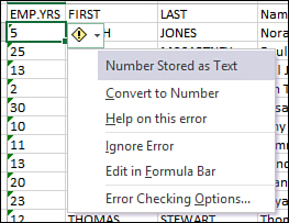
Figure 3.19. With Background Error Checking enabled, Excel informs you if a number is being stored as text.

If you have a worksheet with thousands of cells, it will take a long time to convert them all to numbers. Three options for doing a larger-scale conversion are covered in the next sections.

Using Convert to Number on a Range

One option for converting multiple cells into numbers is to use the information drop-down that Excel has provided:

1. Select the range consisting of all the cells you need to convert (making sure that the first cell in the range needs to be converted). The range can include text and other numerical values, as long as it doesn’t include cells you do not want to be converted to numbers.

2. Click the warning symbol in the first cell.

3. From the drop-down, select Convert to Number, and all cells in the selected range will be modified, turning the numbers to true numbers.

Using Paste Special to Force a Number

If you have the Background Error Checking disabled and don’t see the green warning triangle, try this method for converting cells to numbers:

1. Enter a 1 in a blank cell and copy it.

2. Select the cells containing the numbers, right-click and select Paste Special, Paste Special.

3. From the dialog box that opens, select Multiply, and click OK.

The act of multiplying the values by 1 forces the contents of the cells to become their numerical values.

Using Text to Columns to Convert Text to Numbers

In step 3 of the Text to Columns wizard, you select the data type of a column. You can use this functionality to also correct numbers being stored as text. To convert a column of numbers stored as text to just numbers, follow these steps:

1. Highlight the range of text to be converted.

2. Go to Data, Text to Columns.

3. Click Finish. The numbers are no longer considered numbers stored as text.

Spellchecking Your Sheet

Just like Word, Excel has a spellchecker included. To access it, go to Review, Proofing, Spelling. It reviews all text entries on the sheet. You can configure the options, such as Ignore Words in Uppercase, by clicking the Options button in the Spelling dialog box, or by going to File, Options, Proofing.

If you click the AutoCorrect Options button in the Excel Options dialog box, the AutoCorrect dialog box opens, allowing you to configure how you want the AutoCorrect to work, including automatically replacing text as you type. For example, if you like to abbreviate department as dept. but need it spelled out, you can configure that from this dialog box. Type dept. in the Replace field and department in the With field and click Add. Next time you type dept. in Excel, after you press the spacebar, it will be corrected to department.

Finding Data on Your Sheet

If you press Ctrl+F or go to Home, Editing, Find & Select and select Find from the drop-down, the Find and Replace dialog box opens. Through this dialog box, you can find data anywhere on the sheet or in the workbook. Click on the Replace tab and you can quickly replace the found data.

Click the Options button and the Find dialog box opens up, showing several options to aid in your search, as shown in Figure 3.20:

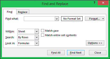
Figure 3.20. Click the Options button to open up the full search potential of the Find and Replace dialog box.

• Within—You can search just the active Sheet or the entire Workbook. You can also narrow Excel’s search by selecting the range before bringing up the dialog box.

• Search—To have the search go down all the rows of one column before going on to the next column, set this to By Rows. To have the search go across all columns in a row before going on to the next row, select By Columns.

• Look In—By default, Excel looks in Formulas, that is, the true value of the data in a cell. When you’ve applied formulas or formatting to a sheet, what you see in a cell might not be what is actually in the cell. Look at Figure 3.21. The value 22.81 is obviously at the top of the column, but a search in Excel does not find it because the value in the cell was calculated. To search for the value, change the drop-down to Values. You can also choose to search in Comments.

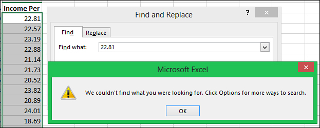
Figure 3.21. If Excel can’t find the number you know is on the sheet, check your settings. If set to Formulas, change to Values and vice versa.

Performing a Wildcard Search

What if you don’t know the exact text you’re looking for? For example, you’re doing a search for Jon Smith but don’t know if Jon was entered correctly. To do a wildcard search, you can use an asterisk (*) to tell Excel there might or might not be additional characters between the n, like this: Jo*n Smith. In this case, Excel would return John Smith, Jon Smith, and Jonathan Smith.

If you have a list of part numbers and can remember all but one of the characters, you can use a question mark (?) to replace the unknown character. Use a ? for each unknown. So if you aren’t sure of the first and last characters, do this: ?482?. This tells Excel that there is definitely one character in each of those positions.

If you need to include a * or ? as part of your search—not as a wildcard, but as actually part of the search text, then precede the symbol with a tilde (~). Doing this tells Excel that the * or ? is not a wildcard character but an actual text character to use in the search.

Using Data Validation to Limit Data Entry in a Cell

Data validation, found under Data, Data Tools, Data Validation, allows you to limit what a user can type in a cell. For example, you can limit users to whole numbers, dates, a list of selections, or a specific range of values. Custom input and error messages can be configured to guide the user entry.

The available validation criteria are as follows:

• Any Value—The default value allowing unrestricted entry.

• Whole Number—Requires a whole number be entered. You can select a comparison value (Between, Not Between, Equal To, and so on) and set the Minimum and Maximum value.

• Decimal—Requires a decimal value be entered. You can select a comparison value (Between, Not Between, Equal To, and so on) and set the Minimum and Maximum value.

• List—Requires user to select from a predefined list, as shown in Figure 3.22. The source can be within the Data Validation dialog box or can be a vertical or horizontal range on any sheet.

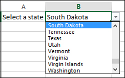
Figure 3.22. Provide users with a list of entries to choose from.

• Date—Requires a date be entered. You can select a comparison value (Between, Not Between, Equal To, and so on) and set the Minimum and Maximum value.

• Time—Requires a time be entered. You can select a comparison value (Between, Not Between, Equal To, and so on) and set the Minimum and Maximum value.

• Text Length—Requires a text value be entered. You can select a comparison value (Between, Not Between, Equal To, and so on) and set the Minimum and Maximum number of characters.

• Custom—Uses a formula to calculate TRUE for valid entries or FALSE for invalid entries.

Limiting User Entry to a Selection from a List

Data validation allows you to create a drop-down in a cell, restricting the user to selecting from a predefined list of values, as shown in Figure 3.22. To set up the source range and configure the data validation cell, follow these steps:

1. Create a vertical or horizontal list of the values to appear in the drop-down. You can place these values in a sheet different from where the drop-down will actually be placed, then hide the sheet, preventing the user from changing the list.

2. Select the cell you want the drop-down to appear in.

3. Go to Data, Data Tools, Data Validation. The Data Validation dialog box opens.

4. From the Allow field of the Settings tab, select List.

5. Place your cursor in the Source field.

6. Select the list you created in step 1, as shown in Figure 3.23. If your list is short, instead of the separate list you created in step 1, you can enter the values separated by commas directly in the Source field. For example, you could enter Yes, No in the source field (no quotes, no equal sign).

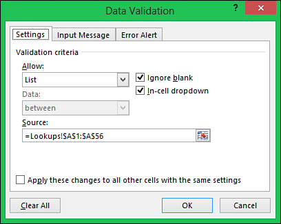
Figure 3.23. The source for the validation list can be a different sheet. You can then hide the sheet from users.

7. If you want to provide the user with an input prompt, go to the Input Message tab and fill in the Title and Input Message fields.

8. If you want to provide the user with an error message, go to the Error Alert tab and fill in the Style, Title, and Error Message fields.

9. Click OK.