10. Subtotals and Grouping

This chapter shows you how data can be summarized and grouped together using Excel’s Subtotal and grouping tools. The ability to group and subtotal data allows you to summarize a long sheet of data to fewer rows. The individual records are still there, so that you can unhide them if you need to investigate a subtotal in detail.

Using the SUBTOTAL Function

The SUBTOTAL function calculates a column of numbers based on the code used in the function. With the correct code, SUBTOTAL can calculate averages, counts, sums, and eight other functions listed in Table 10.1. It can also ignore hidden rows when the 100 version (101, 102, etc.) of the code is used.

Table 10.1. SUBTOTAL Function Numbers

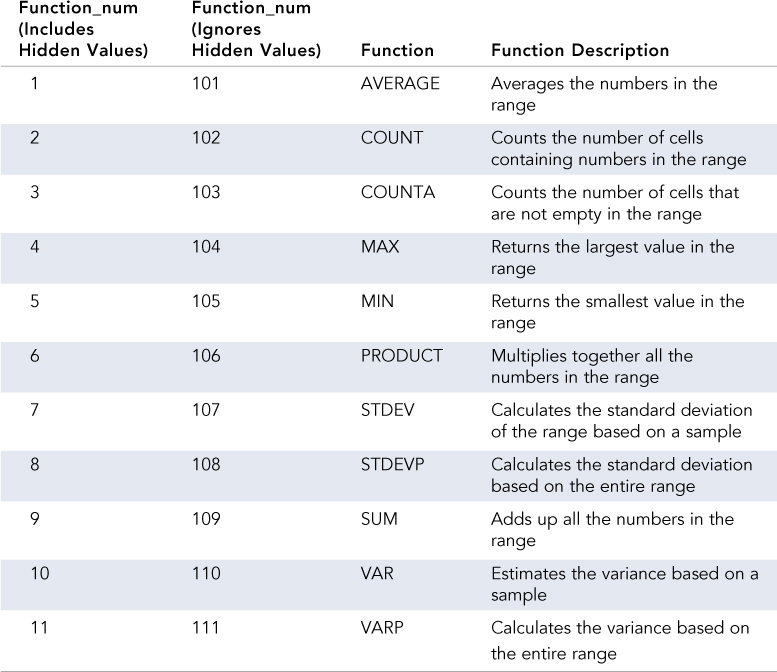
The syntax of the SUBTOTAL function is as follows:

SUBTOTAL(function_num, ref1,[ref2],...)

Figure 10.1 shows the SUBTOTAL function in action versus the SUM function. The SUBTOTAL function with a code of 109 ignores any cells in the range that include SUBTOTAL functions themselves, as shown in the Grand Total. Column E uses the SUM function instead of SUBTOTAL and does not ignore the hidden rows or previous SUM formulas in the Grand Total.

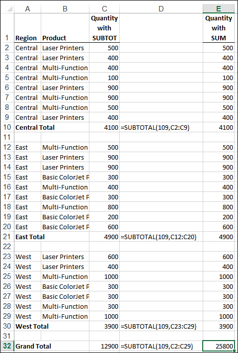
Figure 10.1. SUBTOTAL can ignore hidden rows and other SUBTOTAL calculations, as shown in the Grand Total. The SUM function adds up all data in its range.

Summarizing Data Using the Subtotal Tool

The SUBTOTAL function is very useful, but if you have a large data set, it can be time consuming to insert all the Total rows. When your data set is large, use the Subtotal tool from the Data tab in the Outline group. This tool groups the sorted data, applying the selected function.

From the Subtotal dialog box, shown in Figure 10.2, you can select the column to group the data by, the function to subtotal by, and which columns to apply the subtotal to.

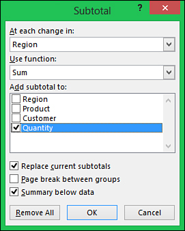
Figure 10.2. Use the Subtotal tool to group data and apply subtotals to specific columns.

Figure 10.3 shows a report where the quantity sold was summarized by region. When data is subtotaled with this method, group/ungroup buttons are added along the row headers. You can use the (-) buttons to group the data rows together, showing only the Total, as was done for the Central region. Click a (+) button to expand the data. To create the report shown in Figure 10.3, follow these steps:

1. Sort the data by the column the summary should be based on, the Region column.

2. Select a cell in the data set.

3. Go to Data, Outline, Subtotal. The Subtotal dialog box, shown in Figure 10.2, opens.

4. From the At Each Change In field, select the column by which to summarize the data, Region.

5. From the Use Function field, select the function to calculate the totals by. Because we want to sum the quantities, choose SUM, but there are many functions to choose from.

6. From the Add Subtotal To field, select the column(s) the totals should be added to, Quantity. Notice that, by default, the last column is already selected.

7. Click OK. The data is grouped and subtotaled, with a grand total at the very bottom.

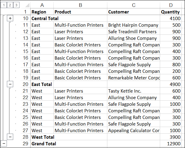
Figure 10.3. Use the Subtotal tool to quickly summarize the quantity by region. You can then group the data, showing only the Total rows, like the Central Total.

Placing Subtotals Above the Data

By default, subtotals appear below the data being summarized. If the subtotals need to appear above the data instead, deselect Summary Below Data in the Subtotal dialog box. This also places the Grand Total row at the top of the data, directly below the headings.

Expanding and Collapsing Subtotals

When data is grouped and subtotaled, outline symbols appear to the left of the row headings, as shown in Figure 10.3. Click the numbered icons at the top (1,2,3 in Figure 10.3) to hide and unhide the data in the sheet. For example, clicking the 2 hides the data rows, showing only the Total and Grand Total rows. Clicking the 1 hides the Total rows, showing only the Grand Total. Clicking the 3 unhides all the rows.

Below the numbered icons, next to each Total and Grand Total, are the expand (+) and collapse (-) icons. These expand or collapse the selected group.

Removing Subtotals or Groups

To remove all the subtotals and groups, click the Remove All button in the Subtotal dialog box. To remove only the group and outline buttons, leaving the subtotal row intact, select Data, Outline, Ungroup, Clear Outline. You can also use Ctrl+8 to toggle the visibility of the outline buttons.

Copying the Subtotals to a New Location

If you hide the data rows, copy all the Subtotal rows and paste them to another sheet. All the data, including the hidden data rows, will appear in the new sheet. To copy and paste only the subtotals, follow these steps to select only the visible cells:

1. Click the Outline icon so that only the rows to copy are visible.

2. Select the entire data set. If the headers are to be included, this can be quickly done by selecting a single cell in the data set and pressing Ctrl+A.

3. Go to Home, Editing, Find & Select, Go to Special, and select Visible Cells Only, as shown in Figure 10.4. Note: The dashed lines in the figure are shown for emphasis only. They will appear in the next step.

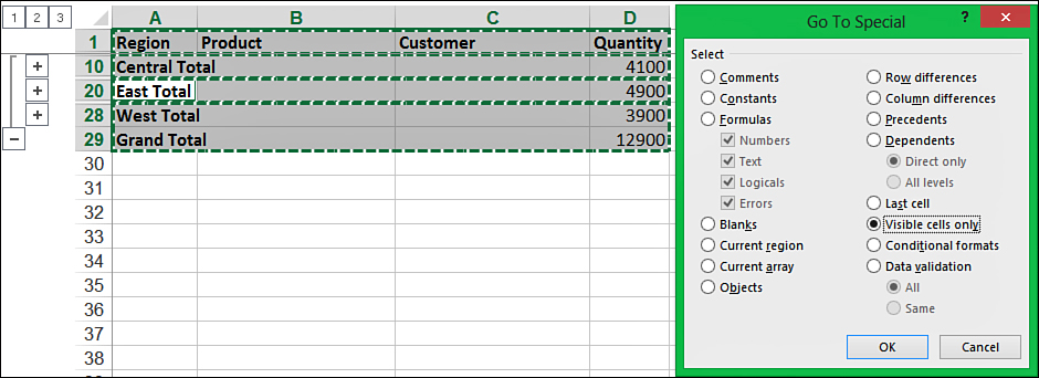
Figure 10.4. Select Visible Cells Only to copy and paste only the Total rows.

4. Select Home, Clipboard, Copy.

5. Select the cell where the data is to be pasted.

6. Select Home, Clipboard, Paste. The SUBTOTAL formulas are converted to values automatically.

Formatting the Subtotals

If you hide the data rows, select the subtotal rows, and apply formatting to them, all the data, including the hidden data rows, will reflect the new formatting. To format just the subtotals, follow these steps to select only the visible cells:

1. Click the Outline icon so that only the rows to copy are visible.

2. Select the entire data set. If the headers are to be included, this can be quickly done by selecting a single cell in the data set and pressing Ctrl+A.

3. Go to Home, Editing, Find & Select, Go to Special, and select Visible Cells Only, as shown in Figure 10.4.

4. Apply the desired formatting.

Applying Different Subtotal Function Types

A data set can have more than one type of subtotal applied to it—for example, a sum subtotal of one column and a count subtotal of another. Because you can only select one function at a time, you will have to use the Subtotal dialog box multiple times. Make sure the Replace Current Subtotals option in the dialog box is deselected so that each subtotal will be applied; otherwise, the previous subtotal(s) will be cleared before the new function is applied. Each subtotal will be calculated and placed on its own row, pushing any existing subtotal rows down, as shown in Figure 10.5 where the Quantity total was added before the Revenue average.

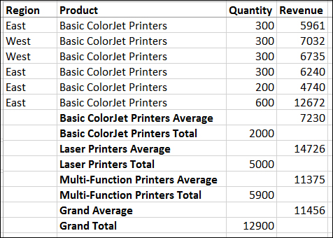
Figure 10.5. You can subtotal multiple columns, mixing different Subtotal function types.

To create the report in Figure 10.5 where, for each change in product, the Quantity column is summed and the Revenue column is averaged, follow these steps:

1. Sort the data by the column the summary should be based on, column B.

2. Select a cell in the data set.

3. Go to Data, Outline, Subtotal.

4. From the At Each Change In field, select the column, Product, by which to summarize the data.

5. From the Use Function field, select the function, SUM, to calculate the totals by.

6. From the Add Subtotal To field, select the Quantity column the total should be added to. Notice that, by default, the last column is already selected and you may have to deselect it.

7. Click OK.

8. Go to Data, Outline, Subtotal.

9. Deselect Replace Current Subtotals.

10. Repeat steps 4 to 6, selecting a new function, AVERAGE, from the Use Function field and a new column, Revenue, to apply the subtotal to. Be sure to deselect the previously selected column, Quantity.

11. Click OK. The data set reflects two subtotals.

Combining Multiple Subtotal Results to One Row

When applying multiple function types, Excel places each subtotal on its own row, as shown in Figure 10.5. There is no built-in option to have the subtotals appear on the same row. But you can manipulate Excel to make this happen by including the column when you apply subtotals to other columns and then manually changing the formula to use the subtotal code actually needed.

The report in Figure 10.6 sums the Quantity, Revenue, COGS, and Profit columns, but has a count of the Customer column.

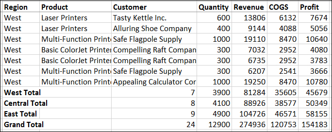
Figure 10.6. Columns D:G are sums of the grouped data, but column C is a count of the data.

To have multiple function types appear on a single row, follow these steps:

1. Sort the data by the column the summary should be based on, the Region column.

2. Select a cell in the data set.

3. Go to Data, Outline, Subtotal.

4. From the At Each Change In field, select the column you want to summarize data by, Region.

5. From the Use Function field, select the function to calculate the majority of totals by, SUM.

6. From the Add Subtotal To field, select the columns the totals should be added to. Include the column where you want to apply the second function type, like the Customer column selected in Figure 10.7.

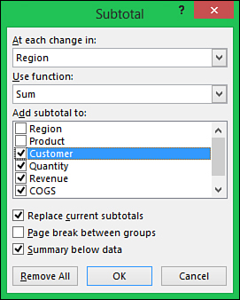
Figure 10.7. The Customer column is selected as a temporary holder for the actual subtotal formula that will be used.

7. Click OK. The Total rows are inserted.

8. Collapse the data set to show only the Total rows by clicking the “2” outline symbol.

9. Select the data in the column where the second function type should be, the Customer column.

10. Go to Home, Editing, Find & Select, Go to Special, and select Visible Cells Only.

11. Go to Home, Editing, Find & Select, Replace.

12. In the Find What field, type (9. 9 is the code for the SUM function that was applied in step 5.

13. In the Replace With field, type the SUBTOTAL function using the desired function number. For example, in Figure 10.8, (3 will replace the SUM function with the COUNTA function.

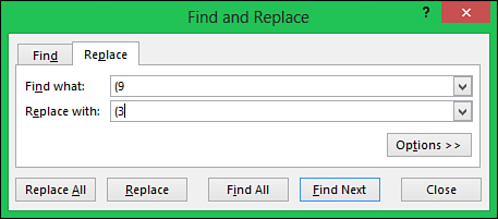
Figure 10.8. Use Find and Replace to replace the automated subtotals with the desired function code.

14. Click Replace All.

15. Click OK to close the Excel notification of the number of replacements made.

16. Click Close. If needed, apply any required formatting to the selected cells.

Subtotaling by Multiple Columns

Figure 10.9 shows a report where the Revenue, COGS, and Profit columns are summed by Region and Product. To subtotal by multiple columns, sort the data set by the desired columns and then apply the subtotals, making sure Replace Current Subtotals is not selected. The subtotals should be applied in order of greatest to least. For example, if the data is sorted by Region, with the products within each region sorted, apply the subtotal to the Region column and then the Product column, like this:

1. Sort the data by the columns the summary should be based on. Because the report is to be by Region then Product, sort by Region first, then Product.

2. Select a cell in the data set.

3. Go to Data, Outline, Subtotal.

4. From the At Each Change In field, select the major column, Region, by which to summarize the data.

5. From the Use Function field, select the function, SUM, to calculate the totals by.

6. From the Add Subtotal To field, select the columns the totals should be added to—Revenue, COGS, Profit.

7. Click OK.

8. Repeat steps 3 to 7 for the secondary column, selecting the minor column, Product, and unselecting Replace Current Subtotals.

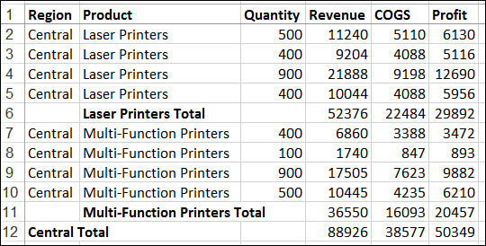
Figure 10.9. Apply subtotals to both Region (the major column) and then Product (the minor column) to get subtotals of both.

Sorting Subtotals

If you try to sort a subtotaled data set while viewing all the data, Excel informs you that to do so will remove all the subtotals. Although the data itself cannot be sorted, the subtotal rows can be, and the grouped data will remain intact. To do this, collapse the data so that only the subtotals are being viewed, and then apply the desired sort.

Adding Space Between Subtotaled Groups

When subtotals are inserted into a data set, only subtotal rows are added between the groups. The report may appear crunched together for some reviewers (see Figure 10.10), and they may request that rows be inserted, separating the subtotaled groups from each other. You can insert extra space into a subtotaled report in two ways.

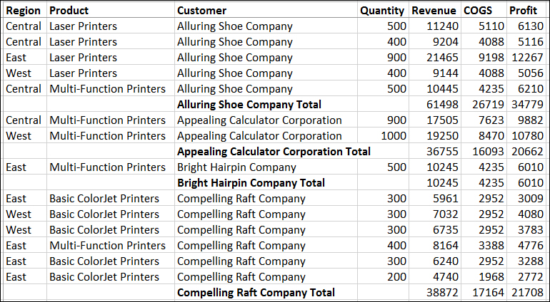
Figure 10.10. The close rows in this report can make it difficult to see the different groups.

Separating Subtotaled Groups for Print

If the report is going to be printed, blank rows probably don’t need to be inserted. Just the illusion needs to be created because the actual need is for more space between the subtotal and the next group. This can be done by adjusting the row height of the subtotal rows. To increase the amount of space when the subtotal is placed below the data, follow these steps:

1. Collapse the data set so that only the subtotals are in view.

2. Select the entire data set, except for the header row.

3. Press Alt+; (semicolon) to select the visible cells only.

4. Go to Home, Cells, Format, and select Row Height.

5. Enter a new value in the Row Height dialog box.

6. Click OK.

7. Go to Home, Alignment, and select the Top Align button.

8. Spacing now appears between each group, as shown in Figure 10.11.

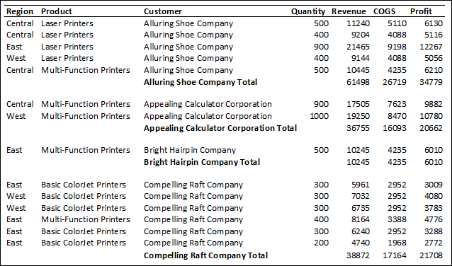
Figure 10.11. Adjust the row height and text alignment of the subtotal rows to separate the groups.

Separating Subtotaled Groups for Distributed Files

It’s a bit involved, but a blank row can be inserted between groups in a file that you’re going to distribute. The method involves using a temporary column to hold the space below where a blank row is needed.

To insert blank rows when subtotals are placed below the data, follow these steps:

1. Collapse the data set so only the subtotals are in view.

2. In a blank column to the right of the data set, select a range as long as the data set.

3. Press Alt+; (semicolon) to select the visible cells only.

4. Type a 1 and press Ctrl+Enter to enter the value in all visible cells.

5. Expand the data set by clicking the outline icon with the largest number.

6. Select the cell above the first cell with a 1 in it.

7. Go to Home, Cells, Insert, Insert Cells.

8. From the Insert dialog box, select Shift Cells Down and click OK, as shown in Figure 10.12. This shifts the 1 one row down.

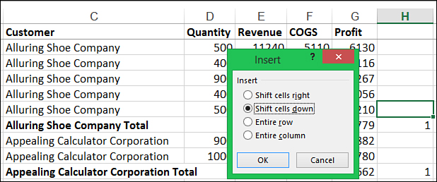
Figure 10.12. Select the cell above the first cell with a 1 in it then insert a new cell to shift all the values in the column down one row.

9. Highlight the column with the 1s in it.

10. Go to Home, Editing, Find & Select, Go to Special.

11. From the Go to Special dialog box, select Constants and click OK.

12. Go to Home, Cells, Insert, Insert Sheet Rows. A blank row is inserted above the row containing a 1.

13. Delete the temporary column.

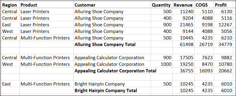
Figure 10.13. Use a temporary column to insert blank rows between groups.

Grouping and Outlining Rows and Columns

Selected rows and columns can be grouped together manually using the options in Data, Outline, Group. This is helpful if you have a sheet designed for multiple users and you want to only show them rows and/or columns specific to the user. Once the data is grouped, an Expand/Collapse button will be placed below the last row in the selection or to the right of the last column in the selection.

If the data to be grouped includes a calculated Total row or column between the groups, you can use the Auto Outline option found in the Group drop-down. This option creates groups based on the location of the rows or columns containing formulas. If the data set contains formulas in both rows and columns, though, the option will create groups for both rows and columns. This tool works best if there are no formulas within the data set itself, unless you do want the groups to be created based off those calculations.

Use the Group option for absolute control of how the rows or columns are grouped. For example, if you have a catalog with products grouped together, users can expand or collapse each group to view the products, as shown in Figure 10.14. By default, the Expand/Collapse buttons will appear below the data. To get them to appear above the grouped data, first apply a subtotal to the data set with Summary Below Data deselected. Then undo the change and apply the desired groupings.

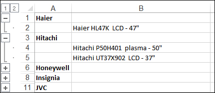
Figure 10.14. Group items together to make it easier for users to view only the desired items.

To manually group rows with the Expand/Collapse button above the grouped data set, follow these steps:

1. Select a cell in the data set.

2. Go to Data, Outline, Subtotal.

3. A message may appear that Excel cannot determine which row has column labels. Click OK.

4. In the Subtotal dialog box, deselect Summary Below Data and click OK.

5. Excel inserts subtotal rows in the data. Click the Undo button in the Quick Access toolbar to remove the rows. While it may appear that you’ve just undone all the previous steps, these steps were required to configure where the outline icon would appear.

6. Select the first set of rows to group together. Do not include the header. For example, to create the Hitachi grouping in Figure 10.14, select rows 4 and 5 to group. To create the Haier group, select only row 2.

7. Go to Data, Outline, Group, Group, or just select the Group button itself.

8. Repeat steps 6 and 7 for each group of rows.

Groups can be cleared one of two ways from the Data, Outline, Ungroup drop-down:

• Ungroup—Ungroups the selected data. Will ungroup a single row from a larger group if that is all that is selected.

• Clear Outline—Clears all groups on a sheet unless more than one cell is selected, in which case the selected item will be ungrouped. If used on data that was subtotaled using the Subtotal button, the subtotals will remain; only the groupings will be removed.