9. Distributing and Printing a Workbook

Once you’re done designing your workbook, you probably want to share it with others. But first, you may want to do a little cleanup, such as adding comments so users can understand what goes in specific fields, hiding sheets you don’t want users to see, or protecting certain cells so users cannot accidently erase your formulas. You can also protect the file so the wrong eyes can’t pry into it.

Once all that’s done, you have to decide how you want to share it. For example, will you print it out, put it on the network and allow multiple users access to it at the same time, or email it? And if you have users with different versions of Excel, such as Excel 2003, you need to ensure those users can access the workbook without a problem. This chapter shows you how to do this and more.

Using Cell Comments to Add Notes to Cells

Cell comments are comments or images you can attach to a cell that appear when a cursor is placed over the cell. By default, the cell comment looks like a yellow sticky note. You can tell if a cell has a comment by the red triangle in the upper-right corner of the cell, as shown in cell A2 of Figure 9.1. Use cell comments to explain to the user what type of data to enter into the cell, explain what the data in the cell is used for, show the user an image of the product being referenced, or any other information you want to convey.

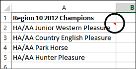
Figure 9.1. Use cell comments to convey additional information to a user without using valuable sheet space.

Inserting and Editing a Cell Comment

To insert a comment, select a cell and go to Review, Comments, New Comment or right-click the cell where the comment should be placed and select Insert Comment. A yellow comment box appears, with the Excel user-defined name already entered to indicate who is entering the comment. If you want, you can delete this text. Otherwise, type the text you want into the comment box. When you’re done, click any cell on the sheet to exit from the comment.

To edit a hidden comment, select the cell and go to Review, Comments, Edit Comment or right-click the comment’s cell and select Edit Comment to make it visible. Your cursor will automatically be placed within the comment box. If the comment is already visible, you can click in the comment box and make changes to the text.

Formatting a Cell Comment

Once you’ve inserted a cell comment, you can format the text and the box or insert an image as the background fill. There are two dialog boxes available when you right-click on a comment and select Format Comment. The first, which you open by right-clicking on the inside of the comment box, only allows you to format the text in the comment. The other opens when you right-click on the comment box while your cursor is a four-headed arrow, as shown in Figure 9.2. It allows you to format the text or box.

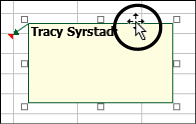
Figure 9.2. Once your cursor changes to a four-headed arrow (shown here), right-click and select Format Comment to format the text or box.

Inserting an Image into a Cell Comment

You can insert an image into a cell comment as a background fill, as shown in Figure 9.3. The image will take up the entire box and resize as you resize the box. You can still type text in the comment and it will appear on top of the image.

Figure 9.3. Insert an image into a cell comment to give the users a visual reference to a label.

To insert an image in a cell comment and change the color of the text so that it shows up over the image, follow these steps:

1. Right-click the cell where you want the comment and select Insert Comment. A cell comment appears with the cursor inside.

2. Place your cursor along any edge of the comment until it turns into a four-headed arrow, then right-click and choose Format Comment. If the Format Comment dialog box that opens only has one tab—Font—close the dialog box and try again. The dialog box that appears should have multiple tabs.

3. Go to the Colors and Lines tab of the Format Comment dialog box.

4. From the Color drop-down in the Fill section, select Fill Effects to open the Fill Effects dialog box.

5. Go to the Picture tab and click the Select Picture button.

6. The Insert Pictures dialog box opens, allowing you to browse for a picture on the computer, at Office.com, anywhere online, or from your SkyDrive. Once you find the image, click Insert and you’ll be returned to the Fill Effects dialog box.

7. Select Lock Picture Aspect Ratio to lock the image ratio. Click OK twice to return to Excel.

8. Resize the comment box if necessary to see the entire image.

9. Highlight the text in the comment box.

10. Right-click within the comment box and select Format Comment.

11. From the Color drop-down of the Font tab, select a new color for the font. Click OK.

Showing and Hiding Cell Comments

A cell comment becomes visible when the cursor passes over the cell then hides again once the cursor is past. If you need the comment to stay open, select the cell and go to Review, Comments, Show/Hide Comment or right-click over the cell and select Show/Hide Comment. If you want to see all the comments on the sheet, go to Review, Comments and click Show All Comments. Select the option again to hide the comment(s).

Deleting a Cell Comment

To delete a comment, select the cell and go to Review, Comments, Delete or right-click over the cell’s comment and select Delete Comment.

Allowing Multiple Users to Edit a Workbook at the Same Time

Excel workbooks are not designed to be accessed by multiple users at the same time. But Microsoft understands that sometimes there is a need for more than one person to edit a workbook at the same time and has provided a limited option. Go to Review, Changes, Share Workbook and the Share Workbook dialog box opens. Select Allow Changes by More Than One User at the Same Time. Go to the Advanced tab to configure how long the change history should be kept, how copies are updated, and how conflicts should be handled. Click OK. Excel prompts you to save the workbook. Click OK to share the workbook.

Sharing a workbook is a double-edged sword. Although it allows for multiple user access, what users can do is severely limited. A shared workbook cannot have Tables, conditional formatting, validation, charts, hyperlinks, subtotals, or scenarios. Users cannot insert or delete rows and columns. Cells cannot be merged and pivot tables cannot be changed. Nor can users write macros or edit array formulas. Basically, only the simplest workbook, such as for data entry, is shareable.

Hiding and Unhiding Sheets

There may be sheets in your workbook that you do not want others to see, such as calculation sheets, data sheets, or sheets with lookup tables. You can hide sheets from users by navigating to the sheet you want to hide and then selecting Home, Format, Hide & Unhide, Hide Sheet. This hides the active sheet—the one you were looking at. You can also hide a sheet by right-clicking on the sheet’s tab and selecting Hide.

To unhide a sheet, go to Home, Format, Hide & Unhide, Unhide Sheet. A dialog box listing all hidden sheets opens. Select the sheet you want to unhide and click Unhide. If you have multiple sheets to unhide, you must repeat these steps for each sheet.

Of course, it’s also possible for a user to open the Unhide dialog box and unhide sheets. To prevent this, you need to protect the workbook. See the “Setting Workbook-Level Protection” section later in this chapter for more information.

Locking Rows or Columns in Place

If you’ve set up your data in a Table, Excel places the Table headings into the column headers when you scroll down the sheet, as shown in Figure 9.4. But normally, when you scroll through a sheet and your data isn’t formatted as a Table, your row and column headings disappear. This can be inconvenient when you have a lot of data and need the identifying headings. With the Freeze Panes options, you can force the top rows, leftmost columns, or both to remain visible as you scroll around the sheet.

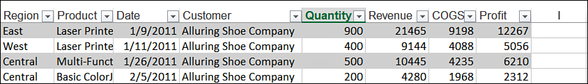
Figure 9.4. Table column headings become part of the column headers so that they are always visible when you scroll down the sheet.

Three options are available under View, Window, Freeze Panes:

• Freeze Panes—Freezes rows and/or columns depending on the cell you have selected at the time. This option changes to Unfreeze Panes if any rows or columns are already frozen.

• Freeze Top Row—Freezes the first visible row of the sheet.

• Freeze First Column—Freezes the first visible column of the sheet.

Freezing Multiple Rows and Columns

The Freeze Top Row and Freeze First Column options allow you to freeze the first row or first column on the sheet; however, if you need to freeze multiple rows and/or columns, you need to use the Freeze Panes option. This option freezes the sheet based on the cell selected when the option is selected. It freezes any rows above and any columns to the left of the selected cell. For example, to freeze row 1 and columns A and B at the same time, select cell C2, then select View, Window, Freeze Panes, Freeze Panes. Now, when you scroll around the sheet, you will always see row 1 and columns A and B.

Clearing Freeze Panes

To turn off the Freeze Panes option, go to View, Window, Freeze Panes, Unfreeze Panes. If you have rows and columns frozen, you can’t choose to unfreeze one or the other. You must unfreeze it all and then refreeze the part you want to keep frozen.

Creating Custom Views of Your Data

View, Workbook View, Custom Views allows you to save the way you have a workbook set up. The hidden rows and columns, filter settings, print settings, and which sheets are hidden are all saved, making it easy to switch between a data entry mode, which shows all your data, and a presentation mode, which hides your calculation sheets.

You have a workbook with a data sheet, a calculation sheet, and a formatted report that needs to be distributed every week after you update it. You want to hide the data and calculation sheets from your viewers. You’ve hidden the sheets, but when it comes time to update them, you have to go through the unhide process twice to unhide both sheets. Instead, create a custom view called Distribution and one called All Data that you can easily switch between as needed, like this:

1. With all sheets unhidden, go to View, Workbook View, Custom Views. The Custom Views dialog box opens.

2. Click Add.

3. Enter a name for the view, such as All Data, in the Name field. If you want the print settings, hidden rows, hidden columns, and filter settings also saved in the view, select the corresponding check box. Click OK.

4. Hide the calculation and data sheets. If you want to hide any rows or columns or set up any filters on the report, do it now.

5. Go to View, Workbook View, Custom Views and click Add.

6. Enter a name for this new view, such as Distribution. If you had any rows or columns hidden, or filter settings, ensure the check box is selected. Click OK.

7. Next time you have to distribute the report, click Distribution before saving. When it’s time to update the workbook, select All Data to show all your sheets.

Configuring the Page Setup

Page setup refers to settings that control how a sheet will look when it is printing. These settings not only include standard print settings, such as the page orientation (portrait or landscape), paper size, and page margins, but they also include settings for the following:

• Repeating specific rows or columns on each printed page

• Printing in black and white

• Printing the gridlines

• Printing 1-2-3 row and A-B-C column headings

• Printing comments

• How cell errors should be displayed

• The order multiple pages should print in (down then over or over then down)

Some of these options are available directly on the Page Layout tab. To access all of these sheet options, go to Page Layout, Page Setup, Print Titles. The Page Setup dialog box opens directly to the Sheet tab, shown in Figure 9.5.

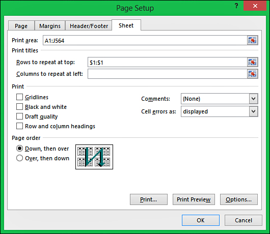
Figure 9.5. Instead of breaking up your table and repeating the heading so that it prints on each page, use the Print Titles option to have Excel automatically copy the row onto each page.

Repeating Rows or Columns on Each Printed Page

When you have a report that spans several pages, you probably want to repeat your row or column headings on all the pages. Follow these steps to have your heading row repeat at the top of each printed page:

1. Go to Page Layout, Page Setup, Print Titles. The Page Setup dialog box opens to the Sheet tab, as shown in Figure 9.5.

2. Click the Collapse Dialog button on the far-right side of the Rows to Repeat at Top field. This minimizes the dialog box and allows you to more easily interact with the sheet.

3. Select the row(s) you want to repeat by clicking the numbered row header(s). You can only select the entire row, not just a few columns of it.

4. Click the button on the far-right side of the Rows to Repeat at Top field to return to the dialog box.

5. Click OK. The selected row(s) will now repeat at the top of each printed page.

Scaling Your Data to Fit a Printed Page

You may find your data is a few rows too long or a few columns too wide to print on a single page. From Page Layout, Scale to Fit, you can adjust the scaling options available to get your data to print as you see fit. These options are also available in the Page Setup dialog box on the Page tab, though the labels are slightly different.

The Width drop-down is useful if you have a few columns going to the next page. From the drop-down, you can choose how many pages you want to force the table to print to. For example, if your report is printing on two pages because you have a column going to the second page, choose 1 page from the drop-down to have Excel adjust the settings, forcing that last column to stay with the others. Similarly, the Height drop-down is used when you have a few too many rows going to another page.

Scale allows you to configure how a sheet will print by setting the percentage of the normal size you want it to print at. 100% is the normal size of the table. Set the percentage to 50% and Excel reduces the size of the table by 50%, allowing for more of it to appear on a sheet, and shrinking the text. Set the percentage to 150% and Excel increases the size of the table and the text.

Creating a Custom Header or Footer

There are two ways you can customize the header or footer. One method is through the Header/Footer tab of the Page Setup dialog box, which you can open using the Page Setup shortcut. Once you’re on the tab, click Custom Header or Custom Footer to design the header or footer. The other method is available when you are viewing your sheet in Page Layout view and you click in the header or footer area, opening the Header & Footer Tools, Design tab. Both provide the same design options, just in a different manner.

The header and footer are unique to each sheet. Each header and footer is broken into three sections: left section, center section, and right section. You can customize each of these three sections in the following ways:

• Add page numbering.

• Add the current date and time.

• Add the file path of the workbook.

• Add the workbook name.

• Add the sheet name.

• Insert text.

• Format any text, including the above options.

• Insert and format an image.

To add one of the options to a section of a header or footer, first select the section, and then click the corresponding button. You can then select the text or image and apply formatting to it.

Adding an Image to the Header and Footer

You can add a company logo to a header so that it appears when printed, instead of taking up space on the computer screen. It’s an easy way to give a report a more professional look. To insert a logo in the header’s left section, as shown in Figure 9.6, follow these steps:

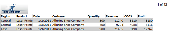
Figure 9.6. Use the header to add a company logo to a printed sheet.

1. Go to View, Workbook View and select Page Layout.

2. As you move your cursor over the area that says “Click to Add Header,” the three sections of the header appear highlighted. Click on the leftmost section. This places your cursor in that section.

3. Go to Header & Footer Tools, Design, Header & Footer Elements, and then click Picture.

4. From the Insert Pictures dialog box, browse or search for the image to import. You can look for images on your local drive, online at Office.com, on the web (you can search through Bing), or on your SkyDrive.

5. When you find the desired image, select it and click Insert.

6. Select Format Picture from the Header & Footer Elements group of the Design tab. Adjust the size on the Size tab. Go to the Picture tab if you need to change the color of the image or crop it. Click OK.

7. Click anywhere outside the header, and the image appears. If you need to modify the image even more, click in the section and repeat step 6.

Adding Page Numbering to the Header and Footer

Page numbering is set up in the header or footer of a sheet. You can show just the page number (1, 2, 3, etc.) or you can show the page number out of the total number of pages, as shown in the right header section in Figure 9.6. If you select multiple sheets when printing, the page numbering will be consecutive for all the sheets in the order they appear in the workbook. (See the “Printing Sheets” section for more information.)

To insert page numbering based on the total number of pages, follow these steps:

1. Go to View, Workbook View and select Page Layout.

2. As you move your cursor over the area that says “Click to Add Header,” the three sections of the header appear highlighted. Click on the rightmost section. This places your cursor in that section.

3. Go to Header & Footer Tools, Design, Header & Footer Elements, and then click Page Number. This places the code for page numbering, &[Page], in the section.

4. You may not see it, but after placing the code, your cursor was placed at the end of the text. So begin typing the following right away: Type a space then the word of followed by another space. Note that you may not see the second space appear.

5. Click Number of Pages. You should now see the following in the section: &[Page] of &[Pages]. Click anywhere outside the footer and you will see the current page number and the total number of pages.

Using Page Break Preview to Set Page Breaks

When in the Page Break Preview viewing mode, you can see where columns and rows will break to print onto other pages. Blue dashed lines signify automatic breaks that Excel places based on settings, such as margins. Blue solid lines are manually set breaks. You can move these lines to set the page breaks where you want by clicking and dragging them to a new location. Follow these steps to change the location of a column break:

1. Select Page Break Preview from the View tab.

2. Place your cursor over the blue column line you want to move until it becomes a double-headed arrow, as shown in Figure 9.7. The line can be solid or dashed.

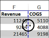
Figure 9.7. Place your cursor over the blue line so the cursor becomes a double-headed arrow.

3. Hold down the mouse button and drag the blue line to where you want the column break to be.

4. Release the mouse button. The dashed blue line becomes a solid blue line, as shown in Figure 9.8.

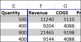
Figure 9.8. After you’ve moved an automatically set column break, it changes from a dashed line to the solid line of a manually set break.

You can also insert additional (row) page breaks by selecting a cell in the row you want to be first on the next printed page, then selecting Page Layout, Page Setup, Breaks, Insert Page Break. A solid blue line appears above the selected cell. To remove a manually inserted page break, select a cell directly beneath the solid blue line and then select Page Layout, Page Setup, Remove Page Break.

Printing Sheets

To print the active sheet, go to File, Print. The Print screen is split in two parts. On the left side are the print settings, such as the number of copies and the printer to print to. On the right side of the screen is a print preview of the sheet. You can move through the pages using the scroll wheel of the mouse, using Page Up and Page Down keys on the keyboard, or using the arrows at the lower left of the Print Preview window. When you’re ready to print, click the Print button on the left side.

If you need to print the entire workbook, open the Print Active Sheets drop-down underneath Settings, shown in Figure 9.9, and select Print Entire Workbook. This prints all visible (unhidden) sheets in the workbook. If you have page numbering setup on the sheets, the numbers will update to show the page’s position in the workbook.

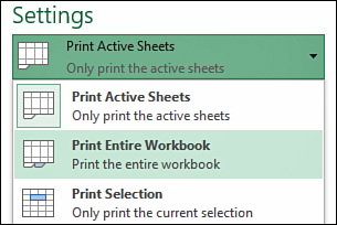
Figure 9.9. Choose to print all visible sheets by selecting Print Entire Workbook.

To print specific sheets, you can hide the sheets you don’t want to print and then use the Print Entire Workbook option. Or, you can use the Ctrl key to select the desired sheets to print. This method doesn’t require you to select a different print option or hide the sheets, yet it also updates the page numbering. For more information on selecting multiple sheets, see the “Selecting Multiple Sheets” section in Chapter 2, “Working with Workbooks, Sheets, Rows, Columns, and Cells.”

Protecting Your Workbook from Unwanted Changes

After spending time setting up a workbook exactly right, you don’t want another user to mess up your hard work. Or, perhaps your workbook contains sensitive data that should only be seen by certain people. Either way, Excel offers various methods of protection you may find useful.

Setting File-Level Protection

Set a password at the file level to prevent an unauthorized user from opening a workbook. You can also allow a user to open the workbook but not save any changes, except as a new file. The permission level is set when the workbook is saved by selecting General Options from the Tools drop-down in the Save As dialog box. From the General Options dialog box, enter a password in the Password to Open field if you want only specific people to be able to open the workbook. If you want anyone to be able to open the workbook but only certain people to make changes, enter a password in the Password to Modify field. Selecting Read-Only Recommended prompts users to open the file as read-only. After clicking OK, Excel prompts you to reenter the password. Once you have completed the save function, the file will be password protected.

To remove the protection, go to the General Options dialog box, clear the fields, and save the workbook.

Setting Workbook-Level Protection

Protection at the workbook level prevents a user from adding, deleting, or moving sheets. To protect the workbook structure, go to Review, Protect Workbook. The Protect Structure and Windows dialog box opens. At the time of writing, there are two options in the dialog box: Structure and Windows. Windows is grayed out. If you deselect Structure, the OK button grays out because without Structure selected, there is nothing to protect. If you want, you can also enter a password. You will have to enter it twice.

Protecting the Data on a Sheet

Protecting a sheet prevents users from changing the content of locked cells. By default, all cells have the locked option selected and you purposefully unlock them (see the following section “Unlocking Cells”). Sheet protection must be applied to each sheet individually.

To protect a sheet, go to Review, Protect Sheet. The Protect Sheet dialog box opens, from which you can select what actions a user can do to the sheet. You can also enter a password. You will have to enter it twice.

Unlocking Cells

While a sheet is still unprotected, you can unlock specific cells so that when the sheet is protected, users can still enter information in the cells you want. To change the protection of selected cells, go to Home, Cells, Format, Format Cells, or right-click on the selection and choose Format Cells. In the Format Cells dialog box, go to the Protection tab and unselect the Locked option. Once you’ve unlocked the desired cells, protect the sheet to protect the other cells.

Allowing Users to Edit Specific Ranges

Unlocking cells and protecting the sheet is an all-or-none solution. That is, none of your users will be able to modify the protected cells unless they can unprotect the sheet first. Suppose you have a form where traveling employees fill in the top half and accounting fills in the bottom half. You want to protect the sheet, so that travelers can’t accidentally fill in the bottom half, but you don’t want to provide the sheet password to accounting so they can fill in the bottom half. Review, Changes, Allow Users to Edit Ranges lets you assign a password to specific ranges, allowing authorized users to edit those ranges.

Figure 9.10 is a travel log. The employee fills out the top table while a member of the accounting department signs off at the bottom. The top table is unlocked for all users but the bottom half, below the “To be filled out by Accounting only” line, is password protected. To apply a password to a selective range while the entire sheet is protected, follow these steps:

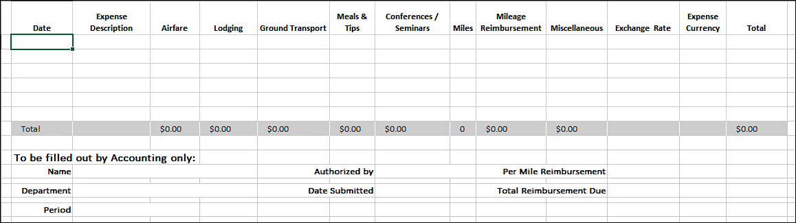
Figure 9.10. Create and protect a sheet that can be used with users of varying permission levels.

1. Ensure the sheet is unprotected.

2. Select the specific accounting only cells: in this example, C11, C13, C15, H11, H13, L11, L13. To select multiple cells, hold down the Ctrl key while you select the cells.

3. Go to Review, Changes, Allow Users to Edit Ranges. The dialog box shown in Figure 9.11 opens.

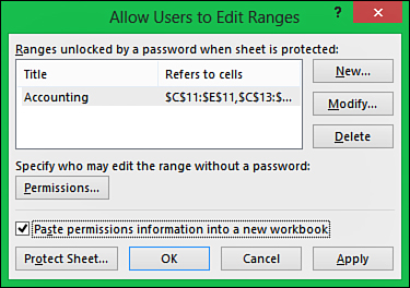
Figure 9.11. Configure Allow Users to Edit Ranges with cells that can be unprotected with a password.

4. Click New. The New Range dialog box opens. Enter a title, such as Accounting. The Refers to Cells already reflects the cells you want to configure. In the Range Password field, enter the password members of the accounting department will use to unprotect those cells.

5. Click OK. Reenter the password to confirm it.

6. If you want to create a log of what you’ve done, check the Paste Permissions Information into a New Workbook check box. When you click OK, the configuration will be logged in a new workbook.

7. If you’re ready to protect the sheet, click the Protect Sheet button.

8. Click OK.

The first time a user tries to enter data in an accounting cell, a password prompt will appear. If the user enters the correct password, the prompt won’t appear again until the workbook is closed and reopened.

Preventing Changes by Marking a File as Final

You can set a workbook as read-only by going to File, Info, Protect Workbook, Mark as Final. This prevents users from accidentally making any changes to the file. When open, a status message appears above the formula bar stating that the workbook is MARKED AS FINAL, but it gives users the option to Edit Anyway. If users click the Edit button, the final status will be lost and they will be able to make changes and save the workbook.

Restricting Access Using IRM

If your organization has configured a Digital Rights Management Server, you can limit your workbook to predefined groups configured by your organization. To enable this option, go to File, Info, Protect Workbook, Restrict Access.

Certifying a Workbook with a Digital Signature

Digital signatures are often used at websites, such as banking sites, to verify their authenticity. You can also add a digital signature to a workbook to authenticate it and prevent others from making changes.

Digital signatures are purchased from third-party certifying authorities. Once you have installed the certificate, go to File, Info, Protect Workbook, Add a Digital Signature. From the Sign dialog box, select the type of signature—created, approved, or both—and enter a reason for signing the workbook. By clicking the Details button, you can provide more information, such as an address. At the bottom of the dialog box is the digital signature Excel found. If it isn’t the correct one, click the Change button to select another.

Once you have your settings entered, click Sign. When users open the workbook, they are notified of the signature. If the user makes changes and saves them, the signature will be removed.

Sharing Files Between Excel Versions

Excel has made many changes over the years. If you plan to send your workbook to users with versions other than Excel 2013, you should ensure that the workbook is compatible with their version(s) of Excel. To do this, go to File, Info, Check for Issues, Check Compatibility. From the dialog box, shown in Figure 9.12, you can select the version(s) to test from the Select Versions to Show drop-down. If there are any compatibility issues, they appear in the box below the drop-down, with a brief explanation and the versions affected. You can decide if it’s an issue you need to resolve, such as a function not available in previous versions of Excel, or one you can safely ignore, such as a new color in Excel. Excel also gives its opinion on whether the issue is significant or minor. If a Find link appears next to the issue, Excel takes you directly to the issue when you click the link.

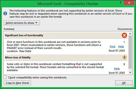
Figure 9.12. Use the Compatibility Checker to verify your workbook will open properly in earlier versions of Excel.

Removing Hidden or Confidential Information

An Excel workbook can hide data in various places such as document properties, cell comments, and hidden rows. The Document Inspector can find much of this information and help you remove it. To run the inspector, go to File, Info, Check for Issues, Inspect Document. After Excel warns you that it could remove important data and that it’s important to save first, the Document Inspector dialog box opens. You can choose the type of content you want the inspector to look for. When you click Inspect, a report of what Excel has found appears by the selected content, as shown in Figure 9.13. You can then choose whether to let Excel remove the content.

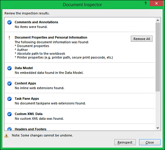
Figure 9.13. Use the Document Inspector to remove information you don’t want to share, such as your name.

Recovering Lost Changes

If you’ve ever closed a file without saving it or had a power failure—this option might be the lifesaver you’re looking for. Excel automatically creates backups of your workbook as you work on it. Depending on its configuration, it also saves a copy of your workbook if you close it without saving.

To check your settings, go to File, Options. From the Excel Options dialog box, go to the Save tab. Under Save Workbooks, ensure that Save AutoRecover Information Every 10 Minutes is selected. This tells Excel to create backups of your workbooks. Set the number of minutes to a time frame that will work best for all of your workbooks.

When Save AutoRecover is selected, the Keep the Last Autosaved Version If I Close Without Saving option becomes available. Select this option and Excel saves the last backup copy it made if you close the workbook without saving. To recover this backup, open the original workbook. Then go to File, Info and by the Manage Versions drop-down, if Excel has a copy saved, it informs you, as shown in Figure 9.14. Click the icon below Versions and Excel opens the file. Review the file, and if you want to keep the work, click the Restore button in the status message above the formula bar. Excel then overwrites the original workbook with this restored version.

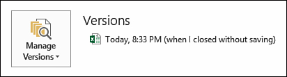
Figure 9.14. Closing without saving doesn’t have to be the end of the world. Excel has settings to automatically back up and recover your work.

Excel won’t keep the autorecover files forever. The backed-up copies of the workbook will be deleted under the following circumstances:

• When the file is manually saved

• When the file is saved with a new filename

• If you turn off autorecover for the workbook (refer to the following Tip)

• If you deselect Save AutoRecover in Excel Options

• When you close the file

• When you quit Excel

Sending an Excel File as an Attachment

You can email your workbook right from Excel by going to File, Share, Email and selecting the format you want to send it in. Once you select an option, Excel generates an email message with the file attached. You just need to fill in the rest of the information and send the message with the file.

Keep in mind that the Outlook window you see isn’t a normal one. It’s the Excel version, and while it’s open, you won’t be able to access the real Outlook window. If you need to get into Outlook, click the Save icon in the message’s Quick Access Toolbar and close the message by clicking the X in the upper-right corner of the window. It will be saved to the Drafts folder in Outlook. You can do what’s needed in Outlook then go to the Drafts folder, open the saved message, and continue emailing your file.

Sharing a File Online

You don’t need to email a file or save it to a network to share it with others. Microsoft offers space on SkyDrive, a place online where you can save your file and give others access to it. You can save your file to your SkyDrive account by going to File, Save As and choosing your SkyDrive from the Places list. For more information on creating a workbook to share on SkyDrive, see Chapter 16.