2. Working with Workbooks, Sheets, Rows, Columns, and Cells

An Excel file is called a workbook and each workbook can contain one or more sheets. This chapter shows you how to create workbooks from scratch or from templates. It shows you how to add, delete, and move sheets within a workbook or between workbooks.

Even a well-planned-out sheet layout may be missing something, such as a date column. Or you might change your mind in the middle of the design, deciding that you want a table elsewhere on a sheet. Instead of starting over, this chapter shows you how to insert rows or columns and move your tables to a new location on your sheet.

Managing Workbooks

Workbook is another name for an Excel file. It’s the workbook you open, save, and close. This section shows you how to create a new workbook, open an existing workbook, and save and close a workbook.

Creating a New Workbook

When you open Excel, it already makes a new workbook available (if the Start screen is disabled) or you can create one by clicking Blank Workbook from the Start screen (if the Start screen in enabled). To create a new workbook if you already have another workbook open, you can click File, New and then click on Blank Workbook, or you can press Ctrl+N.

Opening an Existing Workbook

If the Start screen is turned on, when you open Excel you will see various template icons on the right side of the window and a list of recent workbooks and the option to Open Other Workbooks on the left side of the window, as shown in Figure 2.1.

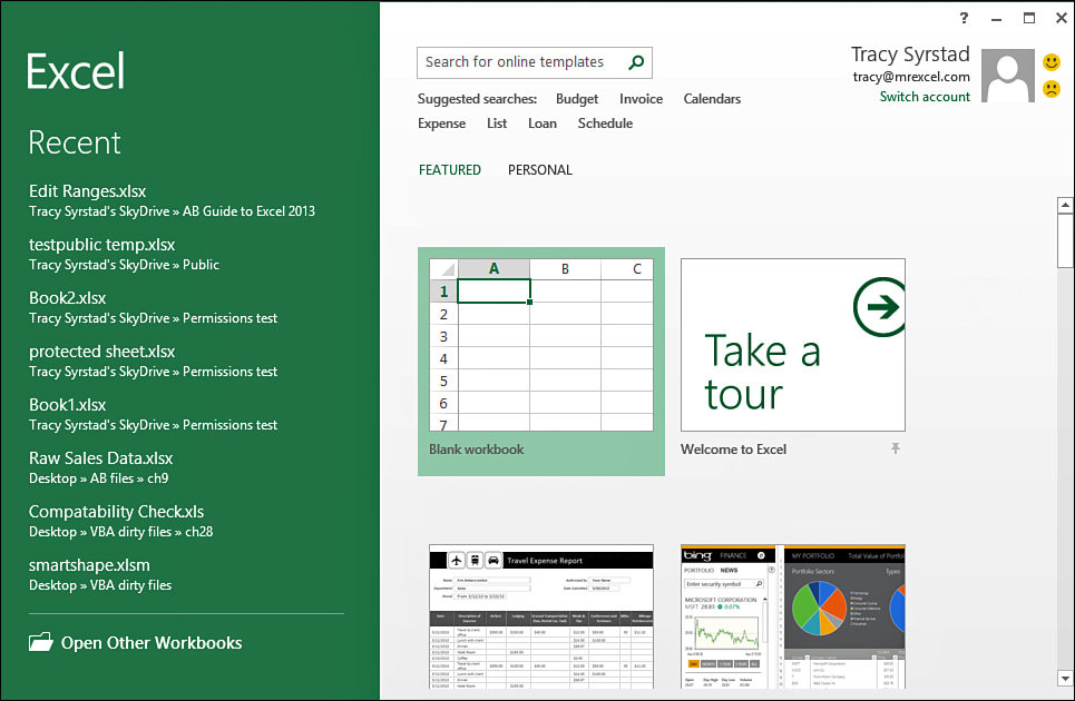
Figure 2.1. The left side of the Start screen lists recently opened workbooks. The right side shows various templates you can start working with.

If you want to open a workbook that was recently open, select it from the list on the left. Notice that the Recent Workbooks list shows the workbook name and its location. See the section “Using the Recent Workbooks list” for information on keeping a workbook in the list.

If the workbook you are looking for is not listed, select Open Other Workbooks. A new window opens in which you can choose the place where the workbook is located, as shown in Figure 2.2. The default places are as follows:

• Recent Workbooks—The most recently opened workbooks and any workbooks you have pinned to the list

• Your SkyDrive—A location on the Internet on Microsoft’s SkyDrive server

• Computer—Your local computer and any networks attached

• Add a Place—A new location you can add, such as a network drive, so it is readily available

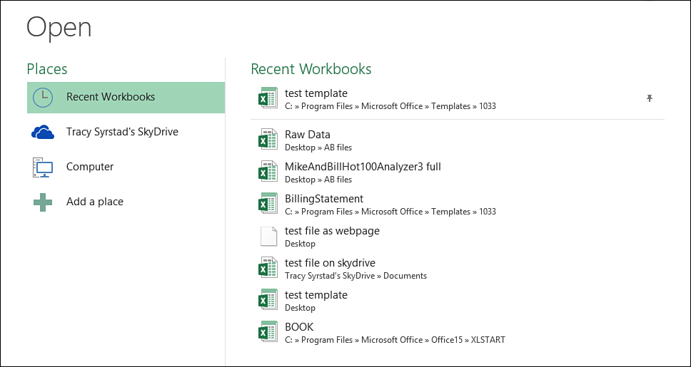
Figure 2.2. Excel makes it easy to share your workbook online with access to your SkyDrive and Microsoft’s online server, or you can save it to your local drive or network.

The area to the right of the Places list will update to reflect your places selection. For the SkyDrive and Computer options, recent folders will be listed, or you can browse to another folder.

When you select a folder or the Browse option, the Open dialog box, shown in Figure 2.3, appears, allowing you to search for a specific Excel file and offering multiple ways to open it.

Figure 2.3. The Open dialog box offers multiple options to search for a specific file.

In the upper-right corner of the dialog box is a Search field in which you can enter terms to search the current folder and its subfolders. Type in a keyword and press Enter.

Excel can open a variety of files, both Excel files and non-Excel. To change the file type, click All Excel Files and a drop-down of other file types appears.

Once you’ve found the file you want to open, you can choose how Excel should open it. By default, Excel opens the file normally, but you can also choose to open it as read-only, as a copy, and more:

• Open—Opens the workbook normally.

• Open Read-Only—Opens a read-only copy of the workbook. You must save the workbook with a different filename if you want to save any changes.

• Open as Copy—Opens as a new copy of the workbook. Excel appends “Copy” to the beginning of the filename.

• Open in Browser—Opens a workbook saved as a web page in your browser.

• Open in Protected View—Opens in Protected view, allowing you to only view the workbook. To make changes, you have to click the Enable Editing button that appears in the alert bar at the top of the sheet.

• Open and Repair—Performs checks while opening the workbook and tries to repair any issues it finds. Or, Excel tries to extract the formulas and values.

Using the Recent Workbooks List

When you go to File, Open a list of workbooks recently opened is shown. The Recent Workbooks list makes it easy to open files you’re currently working on. A pushpin appears when you place your cursor over a workbook listed under Recent Workbooks. The pushpin points to the left when not in use, but place your cursor over the pushpin and click and the pushpin will face downward and the workbook will be moved to the top section of the list, as shown in Figure 2.2. A workbook with a pin facing down is stuck—that is, the workbook will not be removed from the list of recent workbooks until you unstick it by clicking the pushpin again.

Saving a Workbook

When you click the File menu, you see two options for saving your workbook: Save and Save As. Selecting Save saves the workbook with the current name, overwriting the existing file. If the workbook is new and doesn’t have a filename yet, clicking Save opens the Save As dialog box. The Save As dialog box allows you to save a workbook with a new name in a new location. You would select Save to create a copy of the workbook for changes, but want to keep the original workbook intact.

When you select Save As, the area to the right of the File menu changes to show various places where the workbook can be saved to. The default places are as follows:

• Your SkyDrive—A location on the Internet on Microsoft’s SkyDrive server

• Computer—Your local computer and any networks attached

• Add a Place—A new location you can add, such as a network drive, so it is readily available

The area to the right of the Places list updates to reflect recent folders associated with your places selection. You can select from the list or you can browse to another folder, opening the Save As dialog box, as shown in Figure 2.4.

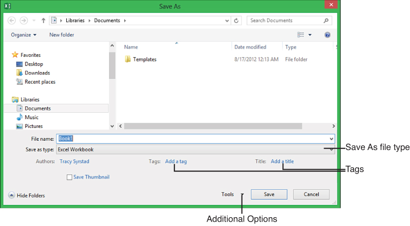
Figure 2.4. The Save As dialog box offers multiple options when saving your workbook.

By default, Excel saves your workbook with an XLSX extension. But if you need to share with Excel 97–2003 users or have macros in your workbook, you must choose another Save As file type. Commonly used extensions are as follows:

• Excel 97–2003 Workbook—XLS: Excel 97–2003 workbook with or without macros

• Excel Workbook—XLSX: Excel 2007–2013 workbook without macros

• Excel Macro-Enabled Workbook—XLSM: Excel 2007–2013 workbook with macros

• PDF—PDF: A Portable Document Format that can be used to distribute your report but prevent users from making changes

Closing a Workbook

When you’re done working with a workbook, you need to close it. To close a workbook, click File, Close or click the X in the upper-right corner. Excel prompts you to save changes if changes have recently been made to the workbook, including recalculating formulas, and the workbook hasn’t been saved. When the final workbook is closed, Excel closes.

Using Templates to Quickly Create New Workbooks

Templates are a great way for keeping data in a uniform design. You could simply design your workbook and reuse it as needed, but if you accidentally save data before you have renamed the file, your blank workbook is no longer clean. When using a template, there’s no risk of saving data in the template because you are working with a copy of the original workbook, not the workbook itself.

Using Microsoft’s Online Templates

Microsoft offers a variety of templates, such as budgets, invoices, and calendars, which can help you get a start on a project. You can search for templates to fit your needs either from the Start screen or by clicking File, New and selecting Featured. A selection of templates appears in the window or you can enter your own keywords in the Search field in the upper left. A search returns matches, which you can filter from a list on the right.

When you click on a template, a preview window opens up, as shown in Figure 2.5. The preview shows a larger example of the template, a brief explanation of its purpose, and how the template has been rated by other users. If you click Create, the template is downloaded (for first-time use) and opened.

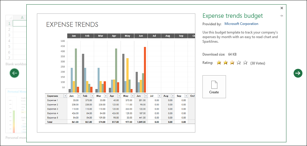
Figure 2.5. Use the left and right arrows in the template preview window to scroll through other available templates before opening one.

Opening a Locally Saved Template to Enter Data

There are multiple ways to open a template to enter data and you can use the method that is most convenient to you. To open a template to create a new workbook, use one of the following methods:

• Double-click the file from its saved location.

• From its saved location, right-click the file and select New.

• Click File, New and select the template from the list of online templates.

• Click File, New, Personal and select from the list of templates saved locally. See the “Saving a Template” section for details on how to configure the location. The Personal option will not appear unless the location is set up.

Opening a Locally Saved Template to Make Changes to the Design

If you need to make changes to the design of a template, the previous methods for opening a copy of the template won’t work. If you do open a template using one of those methods and make changes, you must use the Save As option and save it as a new template. Instead, to open the original template to make changes, use one of the following methods:

• Right-click the file and select Open.

• Click File, Open, select the file and click Open.

Saving a Template

Before you can use your own template or one provided to you and not downloaded from the Office Store, you have to configure where your templates will be stored. This will be a folder where you will place all your templates you want to access through the File, New, Personal dialog box. To set up the location, click File, Options, Save and enter the path in the Default Personal Templates Location field. Once you have a location configured, Personal will appear to the right of Featured. Featured shows Microsoft’s online templates; Personal shows templates in the locally configured location.

Customizing All Future Workbooks

Excel’s default template is fine to start with, but what if there are changes you always make, like changing the margins or the font on the sheet? There isn’t a template file you can overwrite with your preferred adjustments. But if you design your template and save it with a specific name in a specific location, Excel will use it instead of its own template when you create a new workbook. To change the default template used by Excel, follow these steps:

1. Open a blank workbook and make the desired changes.

2. Click File, Save As, Computer and browse to the XLSTART folder. The location is based on where Office was installed. The default location for 64-bit Office is: C:Program FilesMicrosoft OfficeOffice15XLSTART.

3. Enter BOOK in the File Name text box.

4. Select Excel Template as the Save As Type.

5. Click Save. Now, the next time you create a new workbook from scratch, your custom template will be used.

Working with Sheets and Tabs

A sheet, also known as a spreadsheet or worksheet, is where you enter all your data in Excel. A workbook can have multiple sheets—the number limited only by the power of the computer opening the workbook.

Each sheet has a tab, visible above the status bar, as shown in Figure 2.6. The sheet with data that you’re looking at is considered the active sheet. To select another sheet, click on its tab.

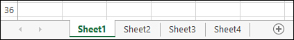
Figure 2.6. The font of the sheet tab you are working on, Sheet1, is bold compared with the other sheet tabs.

Inserting a New Sheet

The quickest way to add a new sheet to a workbook is to click on the circle with a plus sign that appears to the right of the rightmost sheet tab. This inserts a new sheet to the right of the active sheet.

To insert a new sheet to the left of a specific sheet, select the sheet (refer to the “Activating Another Sheet” section) and click Home, Insert, Insert Sheet.

A third method is to right-click on the tab to the right of where you want the new sheet to appear. From the menu, select Insert, select Worksheet, and click OK. The new sheet appears to the left of the tab you right-clicked on, as shown in Figure 2.7.

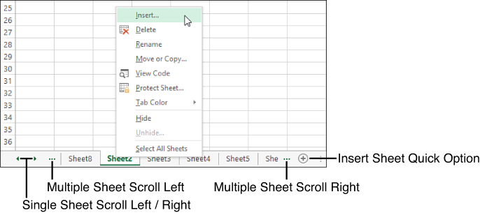
Figure 2.7. You can control where a new sheet is inserted by right-clicking on a tab and selecting Insert. In the figure, the new sheet, Sheet8, appears to the left of the selected Sheet2.

Activating Another Sheet

To activate another sheet, click on its tab along the bottom of the Excel window. You can also navigate sheet to sheet using the keyboard. Ctrl+Page Up selects the sheet to the left; Ctrl+Page Down selects the sheet to the right.

If you have more sheets than can fit in the tab area, three small dots will appear on the left and right side of the area, to show there are more sheets available to view, as shown in Figure 2.7. Clicking on the three dots quickly scrolls through multiple sheets. If instead, you need to scroll one sheet at a time, click the left and right arrows located to the left of the sheet tab area.

If you right-click on the left and right arrows instead, a list of all sheets in the workbook appears. You can then select a sheet, click OK, and you’ll go straight to that sheet.

Selecting Multiple Sheets

You can select multiple sheets at one time. This doesn’t activate them all at once. It groups them together so that an action on one, such as changing the tab color, affects all of them.

To select multiple sheets, select the first one, then while holding down the Ctrl key, select the tabs for the others. As you select each sheet tab, the sheet name will become bold.

To ungroup the sheets, you can either select any sheet other than the active sheet or right-click on any tab and select Ungroup Sheets.

Deleting a Sheet

If you no longer need a sheet, you can delete it, getting it out of your way and reducing the size of your workbook. To delete a sheet, right-click on the sheet’s tab and select Delete. You can also delete a sheet by making it your active sheet and clicking Home, Cells, Delete and selecting Delete Sheet from the drop-down. If there is data on the sheet, a prompt appears to verify this is the action you want to take.

Moving or Copying Sheets Within the Same Workbook

You might want to reorganize sheets within the current workbook to group similar sheets together. Or you might need to copy a sheet to run tests on the data but don’t want to change the original. To move a sheet within a workbook, use the Move or Copy Sheet option found under Home, Cells, Format. The dialog box can also be accessed by right-clicking on a sheet tab and selecting Move or Copy.

In the Move or Copy dialog box, shown in Figure 2.8, make sure the To Book field is the current workbook. If you’re making a copy of the sheet, select the Create a Copy box. Then, in the Before Sheet dialog box, select the sheet you want the active sheet to be placed in front of (to the left of). You can also reorganize the sheets in a workbook by clicking, holding the mouse button down, and dragging the sheet’s tab to a new location. If you want to copy the sheet, hold down the Ctrl key as you move the sheet tab.

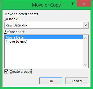
Figure 2.8. The Move or Copy dialog box allows you to copy or move sheets within a workbook or between two different workbooks.

Moving or Copying Sheets Between Workbooks

Many database programs will export data to an Excel workbook or compatible file but might not let you choose an existing workbook to export to. If you have a report workbook designed in which you need the new data, you can copy or move the exported data from its workbook to your report workbook. To move a sheet to a new workbook, use the Move or Copy Sheet option found under Home, Cells, Format. The dialog box can also be accessed by right-clicking on a sheet tab and selecting Move or Copy.

To move or copy a sheet to another workbook, the second workbook must already be open. Make sure the sheet you want to move or copy is the active sheet. Then, using the Move or Copy dialog box, shown in Figure 2.8, select from the To Book field the workbook to move or copy the sheet to. If you’re making a copy of the sheet, select the Create a Copy box. In the Before Sheet dialog box, select the sheet you want the active sheet to be placed in front of (to the left of).

Renaming a Sheet

Excel’s sheet names, Sheet1, Sheet2, etc., aren’t very descriptive. Also, when you copy a sheet in a workbook that already has a sheet by that name, Excel will copy the sheet name, appending a number to the end of it. For example, if you copy Sheet1 within the same workbook, Excel renames it to Sheet1 (2). To give a sheet a more meaningful name, go to Home, Cells, Format and select Rename Sheet from the drop-down. Excel selects the current sheet name in the sheet’s tab and you can then type in the new name. You can also rename a sheet by right-clicking on the sheet’s tab and selecting Rename.

Coloring a Sheet Tab

If you have several sheets you want to visually group together, you can color their tabs. For example, if you have some sheets that are for data input and others for reports, you could color your data input sheet tabs a light yellow and the report tabs a light blue.

To change the color of a tab, go to Home, Cells, Format, and select Tab Color from the drop-down. A selection of colors appears from which you can select the desired color. The tab color of the active sheet appears as a gradient but fills the entire tab for the other sheets. You can also change the tab color by right-clicking the tab and selecting Tab Color.

Working with Rows and Columns

It’s hard to create the perfect data table the first time around. There’s always something you’ve forgotten, such as the date column. Or maybe you did remember the date column but put it in the wrong place. Thankfully, you don’t have to start over. You can insert, delete, and move entire columns and rows with a few clicks of the mouse.

Selecting an Entire Row or Column

When you select an entire row or column on a sheet, you are selecting beyond what you can see on the sheet. You really do select the entire row or column, and whatever you do to the part you can see affects the entire selection.

To select an entire row, place your cursor on the header until it turns into a single black arrow then click on the header for the row. For example, to select row 5, as shown in Figure 2.9, click on the header 5. To select an entire column, click on the header for the column.

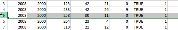
Figure 2.9. Click on the headers to quickly select an entire row or column.

If you need to select multiple, contiguous rows (or columns), click on the first header, then as you hold down the mouse button, drag the mouse down (or up) until you have selected all the rows you need. Let go of the mouse button and perform your desired action on the selection.

If you need to select multiple, noncontiguous rows (or columns), click on the first header, then as you hold down the Ctrl key, carefully click on the headers of the other rows. When done selecting, release the Ctrl key and perform your desired action on the selection.

Inserting an Entire Row and Column

You might want to insert a row if your data table is missing titles over the data. Or, you might need to insert a column if the data table is missing a column of information and you don’t want to enter the information at the end (right side) of the table. When you insert a row, Excel shifts the existing data down. When you insert a column, Excel shifts the existing data to the right.

To insert a new row or column within an existing data set, select a cell in the row or column where you want the inserted row or column to go. For example, if you need to insert a new row 10, select a cell in row 10. Go to Home, Cells. From the Insert drop-down, select Insert Sheet Rows or Insert Sheet Columns. For a shortcut, you can right-click on the row or column header and select Insert, as shown in Figure 2.10.

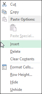
Figure 2.10. Right-clicking a header brings up the options to let you quickly insert or delete a row or column.

Deleting an Entire Row and Column

When you import data from another source, you might need to clean it up by deleting rows or columns of data you don’t need. When deleting a row, Excel shifts the data below the row up. For example, after deleting row 5, what was in row 6 now appears in row 5. If deleting a column, Excel shifts the data that was to the right of the deleted column to the left.

To delete a row or column, select a cell in the row or column to delete and go to Home, Cells and from the Delete drop-down, select Delete Sheet Rows or Delete Sheet Columns. For a shortcut, you can right-click on the row or column header and select Delete, as shown in Figure 2.10.

Moving Entire Rows and Columns

You have to be careful when moving rows and columns. Depending on the method you use, you could end up overwriting other cells. To move rows or columns when you aren’t worried about overwriting existing data, follow these steps:

1. Select the row or column you want to move.

2. The selection is surrounded by a thick line. Place your cursor over the line until it turns into a four-headed arrow, as shown in Figure 2.11.

Figure 2.11. When the cursor changes to a four-headed arrow, you can click and drag the column to a new location.

3. Click on the line and hold the mouse button down.

4. Drag the selection to a new location and let go.

5. If there is any data in the new location, Excel asks if you want to overwrite it. If you say No, the move will be canceled.

6. The original row or column will still be there, but it will be empty.

If you need to keep data in the new location intact, you could insert a row or column in the new location, copy the data to be moved, paste it in the inserted rows or columns and then go back to the original location, select it again, and delete it. Or, you could get it done more quickly by selecting and cutting the row or column, right-clicking on the new location, and selecting Insert Cut Cells. Excel moves the data in the new location, inserting the cut data and also deleting the data in the old location.

To perform these actions using the ribbon, after selecting and cutting the row or column, select a cell in the new location and go to Home, Cells, Insert and select Insert Cut Cells from the drop-down.

Working with Cells

Just like you can insert, move, and delete entire rows and columns, you can also insert, move, and delete cells. This section will show you how to quickly jump to a cell you can’t currently see on your sheet, select noncontiguous ranges, and insert, move, and delete cells.

Selecting a Cell Using the Name Box

Chapter 1, “Understanding the Microsoft Excel Interface,” explained how each cell has an address made up of the column and row it resides in. The basics of navigation were touched upon—you can either click on a cell or use the keyboard to select a cell.

You can also jump to a cell by typing the cell address in the Name box, located above the sheet in the left corner. This is a great way of traveling quickly to a specific location on a large sheet.

To use this method, you must enter the cell address properly—that is, the column then the row. For example, if you want to jump to cell AA33, you must type in AA33; you can’t type in 33AA. After typing the address, press Enter and the currently selected cell will move to cell AA33.

Selecting Noncontiguous Cells and Ranges

In Chapter 1, you were introduced to the basics of cell and range selection in the section “Selecting a Range of Cells.” In this section, you learn how to select multiple, noncontiguous ranges, as shown in Figure 2.12.

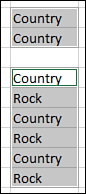
Figure 2.12. You can select noncontiguous cells by holding down the Ctrl key as you select each range.

You don’t always want to select cells right next to each other. For example, you might want to select only the cells with negative values and make them bold. You could select each cell one at a time and apply the bold format, or you could hold down the Ctrl key and select each cell. Once all the cells are selected, then you let go of the Ctrl key and select your desired format (or other action).

Inserting Cells and Ranges

When you insert or delete rows and columns, Excel shifts all the data on the sheet. If you don’t want all the data shifted, select a specific range, then either right-click over the selection and choose Insert or go to Home, Cells, Insert and select Insert Cells from the drop-down. A prompt will appear, asking you in which direction you want to shift your existing data, as shown in Figure 2.13. If you want to insert rows, choose Shift Cells Down. If you want to insert columns, choose Shift Cells Right.

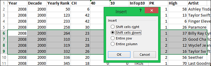
Figure 2.13. You can control how much of a row or column is inserted by selecting a specific range beforehand.

Deleting Cells and Ranges

When you delete a range, you remove the cells from the sheet, shifting other data over to fill in the empty space. If you aren’t careful, you can ruin the careful layout of your sheet, for example, moving data from the credit column to the debit column. If what you really wanted was to delete the data in the cells, leaving the cells intact, Excel calls this clearing the contents. For specifics on clearing contents, see the section “Clearing the Contents of a Cell,” in Chapter 3, “Getting Data onto a Sheet.”

To delete a range from a sheet, select the range and go to Home, Cells, Delete and select Delete Cells from the drop-down. From the Delete dialog box that opens, choose whether you want to Shift Cells Left or Shift Cells Up. You can also open the dialog box by right-clicking on the selected range and choosing Delete from the menu.

Moving Cells and Ranges

You have to be careful when moving a range—you could end up overwriting other cells. If you need to move rows or columns and aren’t worried about overwriting existing data, use the following method. If you don’t want to overwrite existing data in the new location, you need to use the Insert Cells method explained in the section “Inserting Cells and Ranges.” To move rows or columns when you aren’t worried about overwriting existing data, follow these steps:

1. Select the range you want to move.

2. The selection is surrounded by a thick line. Place your cursor over the line until it turns into a four-headed arrow, as shown in Figure 2.14.

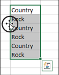
Figure 2.14. Be careful when dragging your selection to a new area as it will overwrite anything there.

3. Click on the line and hold the mouse button down.

4. Drag the selection to a new location and let go.

5. If there is any data in the new location, Excel asks if you want to overwrite it. If you select No, the move will be canceled. Select Yes to complete the move and clear the contents of the original range.