1. Understanding the Microsoft Excel Interface

If you already know how to add a custom tab to the ribbon, select cell D28, or install an add-in, then you’ve probably spent some time using Microsoft Excel. However, if what you’ve just read makes little sense to you, then this chapter is especially for you. This chapter explains the basic parts of the Excel window, how to use them, and the terminology used to refer to them. It also shows you how to navigate around a sheet and how to install add-ins and apps to expand on Excel’s amazing functionality.

Taking a Closer Look at the Excel Window

When you open Excel 2013 for the first time, you should see a window similar to Figure 1.1. It’s a list of templates that you can start off with. Chapter 2, “Working with Workbooks, Sheets, Rows, Columns, and Cells,” covers the details about templates. For now, click once on the Blank Workbook item in the upper-left corner to open a blank spreadsheet, as shown in Figure 1.2.

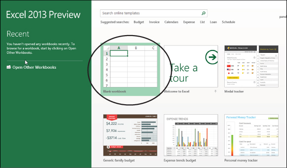
Figure 1.1. Select the Blank Workbook item (circled) to open a blank spreadsheet.

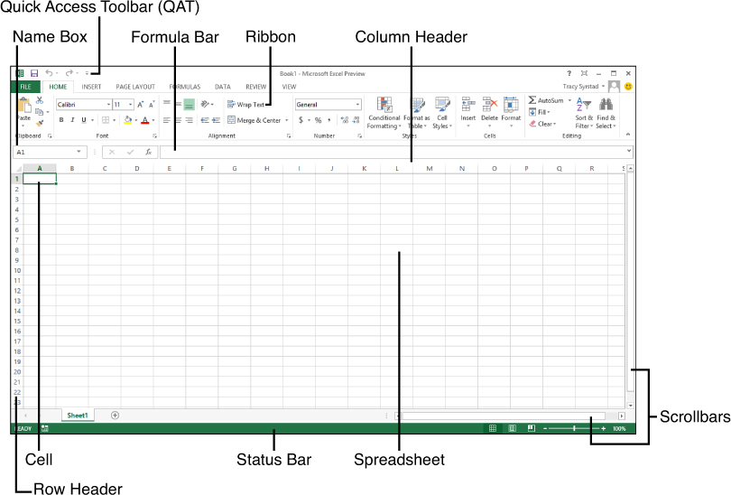
Figure 1.2. The Excel window is made up of many components that you’ll use when working on a spreadsheet.

That big grid taking up most of the Excel window is the spreadsheet, also known as a worksheet or, simply, a sheet. Each little box is a cell. Multiple cells selected together are commonly known as a range.

Right above the grid are letters known as column headers. Down the left side of the grid are numbers, also known as row headers. The intersection of a single column and a single row is a cell. Each cell has an address made up of the column letter then the row number. Figure 1.3 shows cell C8 selected. Note the C in the column header is highlighted as is the 8 in the row header.

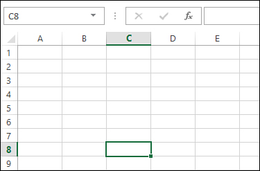
Figure 1.3. The intersection of a column and a row is a cell. The cell gets its name from the column and row headers, in this case C8.

Above the headers and to the left is the Name box. This box shows you what you have selected on the sheet. This can be a cell address, a named range, a table, a chart, or some other object on the sheet. When you first opened Excel, the Name box was likely showing A1. If you’ve selected another cell on the sheet, the address has changed to show that cell’s address, such as C8. Later in this chapter, you learn how you can use the Name box to quickly move to another area of the sheet.

To the right of the Name box is the formula bar, which is a slight misnomer. Although that is probably the most common use of this field, the formula bar actually reflects anything that’s been typed into a cell, not just formulas.

At the top of the Excel window is the ribbon, where you choose what you want to do on your sheet, such as formatting text or inserting a chart. See the section “Making Selections from the Ribbon” for information on the different types of buttons on the ribbon. As you use Excel, you’ll notice new tabs in the ribbon appearing depending on what you’re doing in the sheet area. These tabs are context sensitive—they only appear when they are useful. Other times, they stay out of your way.

The Quick Access Toolbar, also known as the QAT, is located in the upper-left corner of the Excel window. It is always visible, even when the ribbon is minimized and, unlike the ribbon, the commands aren’t dependent on what you are doing in Excel, such as working with a chart.

Below and to the right of the grid are scrollbars, which can be used to move around the sheet. You can either click and drag a bar or use the arrows at either end of the scroll area.

The status bar is along the bottom of the Excel window. Not only does it show the status of Excel, such as Ready or Calculating, on the left side, but it also includes buttons for changing the page view or zoom. In the right corner of the status bar is the Zoom slider. You can use the slider or the - and + buttons to change the zoom of the active sheet.

To the left of the Zoom slider are three buttons for changing how you view the active sheet: Normal, Page Break Preview, and Page Layout. The default view is the Normal view, showing just the sheet.

With Page Break Preview, you can see where columns and rows will break to print onto other pages. Dashed lines signify automatic breaks that Excel places based on settings, such as margins. Solid lines are manually set breaks. See Chapter 9, “Distributing and Printing a Workbook,” for more information on setting and moving page breaks.

The Page Layout view is like an editable Print Preview—you can see what your page will look like when it prints out, but you can still enter data and make other changes. Columns and rows will move between pages as you adjust their widths or the margins of the page. You can also enter information directly into the header and footer of a page. See Chapter 9 for information on adding headers and footers.

Making Selections from the Ribbon

Along the top of the ribbon are tabs (File, Home, Insert, Page Layout, Formulas, Data, Review, View), which you can select to show new options in the ribbon area below the tabs. Each tab consists of multiple groups containing buttons and drop-downs of similar functionality. For example, on the Home tab, you have an Alignment group, which consists of buttons and drop-downs for aligning, wrapping, and merging data.

Some groups have a small arrow in the lower-right corner, as shown in Figure 1.4. Clicking this arrow, the dialog box launcher, opens up a single dialog box with all the options of the group and more. If you can’t find the option you want on the group or you want to use multiple commands (for example, changing the font type and alignment of a cell’s contents), you might want to use the dialog box.

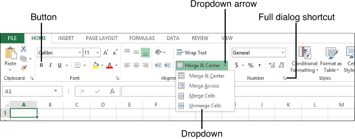
Figure 1.4. The ribbon consists of multiple types of controls.

Arranging Windows So You Can See Multiple Sheets at the Same Time

Sometimes you might want to compare data in two or more workbooks. If you have multiple monitors, you can simply drag an Excel window to another monitor. But if you need to show data side by side on the same monitor, Excel offers two methods. Clicking View, Window, Arrange All opens the Arrange Windows dialog box, which allows you to arrange all the current windows in a Tiled, Horizontal, Vertical, or Cascade view. Clicking View, Window, View Side By Side provides a quick way to view two windows horizontally. You can then select Synchronous Scrolling to lock the scrollbars together and move the data on both sheets at the same time.

Zooming In and Out to Better See Your Data

The ability to zoom in and out on a sheet is an often-forgotten functionality in Excel. Instead, large fonts are used when designing a sheet, then the designer later wonders why there are problems, such as the validation text being too small to see. Instead of relying on font size to make text on the sheet larger, zoom in on the sheet.

There are three ways to change the zoom on a sheet:

• View, Zoom—On the View tab, the Zoom group contains three options for zooming on a sheet:

• Zoom—Brings up the Magnification dialog box

• 100%—Sets the zoom to 100%

• Zoom to Selection—Zooms in on the selected range

• Wheel mouse—While holding down the Ctrl key, use the scroll on your mouse to zoom in and out.

• Zoom slider—In the lower-right corner of the Excel window is the Zoom slider. You can use the slider or the - and + buttons to change the zoom of the active sheet.

Getting to the Built-in Help

There are two ways to bring up the Help interface in Excel. You can press F1 on your keyboard or click the ? icon in the upper-right corner of the Excel window. If an Internet connection is found, you’ll be able to search Microsoft’s online database. Otherwise, your search results will be limited to the Help files on your system.

Once you have the Help dialog box open, you can change your source for help. If you have an Internet connection but would rather use the Help files on your computer, click the arrow to the right of Excel Help and select Excel Help from Your Computer, as shown in Figure 1.5. From then on, search results will be from your computer. You can always switch it back to getting online Help if you don’t find what you need locally by selecting Excel Help from Office.com from the drop-down.

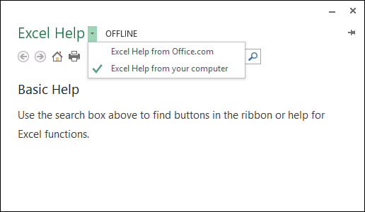
Figure 1.5. You can choose whether to search the online Help or the local Help files.

Troubleshooting the Excel Options

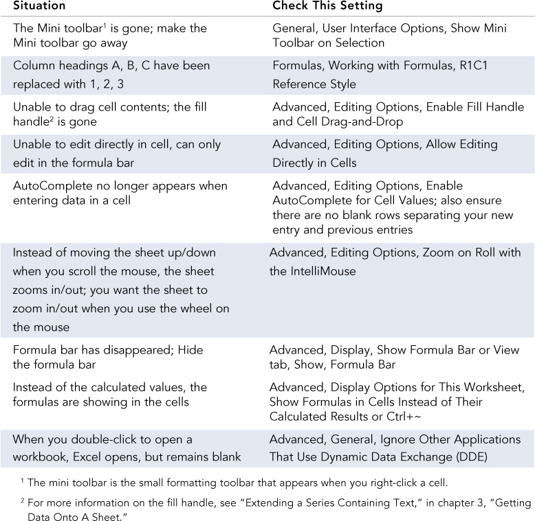
There’s nothing more frustrating than opening Excel and finding out something strange has happened to the way Excel works. Table 1.1 reviews possible scenarios and the settings under File, Options that could be the source of the problem.

Table 1.1. Possible Situations and Solutions

Closing Files and Exiting Excel

To close a file opened in Excel, go to File, Close or click the X in the upper-right corner of the window. This only closes the file. If you have multiple files open, you need to close each one before Excel will close.

Customizing the Excel Window

If you’re using Excel on a tablet, the ribbon can take up a lot of the screen. If you’re entering a long formula in a cell, you might not be able to see enough of it in the formula bar. Or perhaps you want a quicker way of getting to the ribbon options you use the most. In any case, Excel offers multiple customizations to make Excel handier for the way you use it.

Changing the Size of the Formula Bar So You Can See More Data

By default, the formula bar shows a single line, and that’s probably how you’ll want it most of the time, but it can be expanded to show multiple lines. One way is by clicking the down arrow on the far right of the formula bar. This opens the bar to show about three lines of information. Click the arrow again to shrink the field back up to a single line.

The other option allows you more control on how wide the field is. Place the cursor along the bottom of the field until it turns into a double arrow, as shown in Figure 1.6. Press and hold down the mouse button as you drag the field down. Let go of the mouse when you have the field the desired size. To return the field to its normal size, drag it up in the same way you dragged it down or click the arrow on the far right.

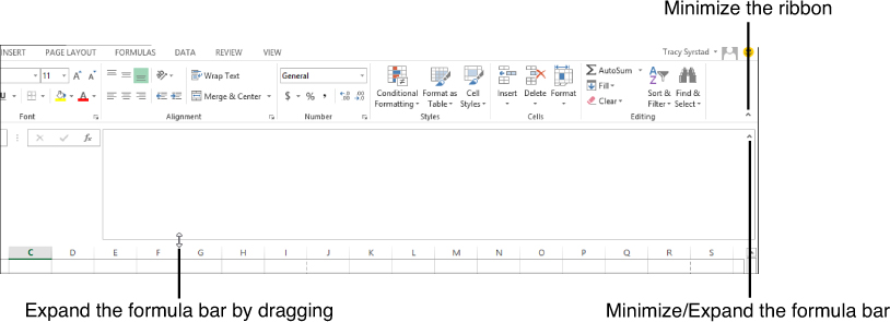
Figure 1.6. You can change the size of the ribbon and formula bar to suit your needs.

Minimizing the Ribbon to Show Only the Tab Names

If you’re working on a system with a small screen, the ribbon probably takes up too much space on the screen. To toggle the ribbon between being minimized and normal, press Ctrl+F1 on the keyboard. You can also minimize the ribbon area by clicking the arrow in the lower-right corner of the ribbon. To set the ribbon back to normal, click on a tab to open up the ribbon, then click on the pin that now appears where the arrow used to be. When minimized, the ribbon will expand when you select a tab and then minimize when you click your mouse elsewhere.

Showing or Hiding Tabs in the Ribbon

Going to File, Options, Customize Ribbon opens the dialog box shown in Figure 1.7. The dialog box allows you to show or hide existing tabs or create your own tabs and groups. You can also open this dialog box by right-clicking on a tab and selecting Customize the Ribbon.

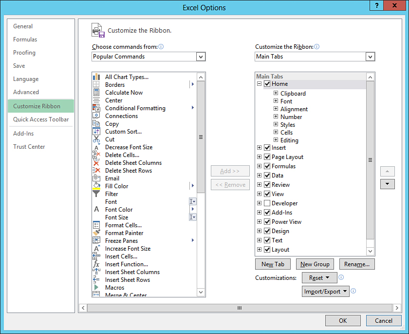
Figure 1.7. Use the Customize the Ribbon dialog box to hide tabs you don’t feel you need or to create tabs with controls you find most useful.

If you have a narrow screen, you might want to hide some tabs so that others can be more easily accessed. To show or hide a tab, follow these steps:

1. Right-click on any tab and select Customize the Ribbon.

2. The list of existing tabs is on the right side of the Customize the Ribbon dialog box.

3. Select or deselect the tab(s) you want shown or hidden from view and then click OK.

Removing a Group from a Tab

You can’t customize the default groups with your own commands, but you can remove the groups, making room for your own custom group on the tab. To remove a group, follow these steps:

1. Right-click on any tab and select Customize the Ribbon.

2. The list of existing tabs is on the right side of the Customize the Ribbon dialog box.

3. Expand the tab containing the group you want to remove.

4. Select the group to remove, right-click it, and select Remove.

Adding More Buttons to the Ribbon

The default tabs and groups in Excel might not be the ones best for you or for a particular situation. You can insert a custom tab into the Main Tabs group or the Tool Tabs group. Once the tab has been added, you can add the groups and buttons most useful to you.

Inserting a New Tab

To create a custom tab in Excel to which you can add groups and buttons that you find most useful, follow these steps:

1. Right-click on any tab and select Customize the Ribbon.

2. Select where you want your tab to be from the list on the right side of the dialog box. The new tab will be placed below your selection.

3. Click New Tab. Excel creates a new tab with a new group, both with (Custom) after the name.

4. Highlight the new group and click Rename to rename the group.

5. Highlight the new tab and click Rename to rename the tab.

Adding a New Group to a Tab

Although not required, grouping similar buttons together can make them easier to find, especially if you’re helping someone else find a specific function. When you create a new tab, Excel automatically adds a new group for you, but you might need another group.

To add a custom group to a tab, follow these steps:

1. Right-click on any tab and select Customize the Ribbon.

2. In the list on the right side of the dialog box, navigate to where you want to add a new group. The new group will be placed below your selection.

3. Click New Group. Excel creates a new group.

4. Highlight the new group and click Rename to rename the group.

Adding a New Button

Excel won’t allow you to add a button to any of the default groups, but there aren’t any such limitations on the custom groups you create. To add a new button to a custom group, follow these steps:

1. Right-click on any tab and select Customize the Ribbon.

2. In the list on the right side of the dialog box, navigate to where you want to add the new button. The new button will be placed below your selection.

3. In the list on the left side of the dialog box, find the button you want to add.

4. Click Add to add the button to the group.

Moving the QAT to Below the Ribbon

You can move the Quick Access Toolbar (QAT) to below the ribbon by clicking on the arrow on the right end of the toolbar and selecting Show Below the Ribbon, as shown in Figure 1.8. If the toolbar is already below the ribbon, the option will be changed to Show Above the Ribbon.

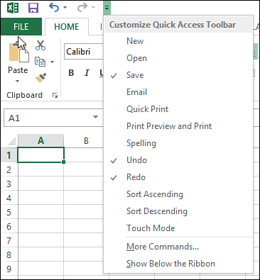
Figure 1.8. Almost any command can be added to the QAT and you can also add some selections from within drop-downs.

Customizing the Commands on the QAT

You can create a custom tab if you have a lot of commands to add, but those commands are only available when the tab is active. If you have options you want available at any time, you can add them to the QAT.

Clicking the arrow on the right end of the QAT opens a list of commonly used commands, as shown in Figure 1.8. Click on one of the options to add it to the QAT. If the command you want isn’t listed, you can select More Commands, which opens the Customize the Quick Access Toolbar dialog box.

There are three ways to customize the QAT:

• Click on the drop-down arrow on the right end of the toolbar and select from the predefined commands.

• Right-click a button on the toolbar and select Customize Quick Access Toolbar to open the Customize the Quick Access Toolbar dialog box.

• Right-click on a command or drop-down item in the ribbon. If the option Add to Quick Access Toolbar appears, select it to add the item to the toolbar.

To add a command to the Quick Access toolbar using the Customize the Quick Access Toolbar dialog box, follow these steps:

1. Click on the drop-down arrow on the right end of the toolbar and select Customize Quick Access Toolbar.

2. Navigate the list on the left side of the dialog box, shown in Figure 1.9, to find the command you want to add to the toolbar.

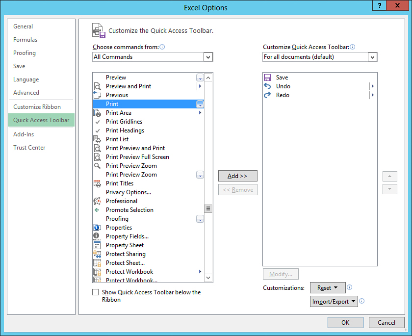
Figure 1.9. Add commands you always want available to the QAT.

3. Select the command and click Add to copy the command to the Quick Access Toolbar.

Customizing the QAT for Just the Current Workbook

You can add commands to the QAT that will appear only when a specific workbook is open. This can be especially useful if your workbook contains macros you want to activate with buttons (for more information on macros, see chapter 15, “An Introduction to Using Macros and UDFs”). To add a macro button to the QAT that only appears when the current workbook is open, follow these steps:

1. Click on the drop-down arrow on the right end of the toolbar and select Customize Quick Access Toolbar.

2. Select the current workbook from the drop-down on the right side of the dialog box.

3. Select Macros from the drop-down on the left side of the dialog box.

4. Select the macro you want to assign to the toolbar and click Add.

5. With the macro selected in the list on the right side of the dialog box, click Modify.

6. Select a symbol for the button and change the Display Name that will appear when the cursor hovers over the button. Click OK.

7. Your custom macro button will appear in the toolbar.

Removing Commands from the QAT

If you decide you no longer require a command on the QAT, you can remove it in one of three ways:

• Click on the drop-down arrow on the right end of the toolbar and deselect the command from the list of predefined commands.

• Click on the drop-down arrow on the right end of the toolbar or right-click any button on the ribbon and select Customize Quick Access Toolbar to open the Customize the Quick Access Toolbar dialog box. Select the command from the list on the right side of the dialog box and click Remove.

• Right-click the command button itself in the Quick Access Toolbar and select Remove from Quick Access Toolbar.

Moving Around and Making Selections on a Sheet

You can move around on a sheet using the mouse or the keyboard, depending on which method is most comfortable for you. To select a cell using the mouse, click on the desired cell. To select a cell using the keyboard, use the navigation arrows on the keyboard. You can also use the number keypad arrows if the NumLock feature is turned off.

Keyboard Shortcuts for Quicker Navigation

Using the navigation arrows on the keyboard can be a little slow, especially if you have a lot of cells between your currently selected cell and the one you want to select. Even using the mouse can take some time to navigate from the top of your data to the bottom. The following list details a few keyboard shortcuts to make navigation a little easier:

• Ctrl+Home jumps to cell A1, located at the upper-left corner of the sheet.

• Ctrl+End jumps to the last row and column in use.

• Ctrl+Left Arrow jumps to the first column with data to the left of the currently selected cell. If there is no data to the left, then it will select a cell in the first column, A.

• Ctrl+Right Arrow jumps to the first column with data to the right of the currently selected cell. If there is no data to the right, then it will select a cell in the last column, XFD.

• Ctrl+Down Arrow jumps to the first row with data below the currently selected cell. If there is no data below the selected cell, it will select a cell in the last row.

• Ctrl+Up Arrow jumps to the first row with data above the currently selected cell. If there is no data above the selected cell, it will select a cell in row 1.

Selecting a Range of Cells

You’ll often find yourself needing to select more than a single cell. For example, if you have text on a sheet you want to apply a new font to, instead of selecting one cell at a time and applying the font, you can select all the cells and then apply the font, as shown in Figure 1.10.

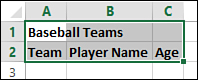
Figure 1.10. The ability to select a range is an important skill to have when working on a sheet.

To select a range using the mouse, follow these steps:

1. Select a cell that will be in the corner of your selection.

2. Hold down the mouse button as you drag the mouse to cover the desired cells.

3. When you get to the last cell, let go of the mouse button. You will have selected a range similar to what is shown in Figure 1.10.

4. As long as you don’t click elsewhere on the sheet, the range will remain selected.

To select a range using the keyboard, follow these steps:

1. Select a cell that will be in the corner of your selection.

2. Press F8 on the keyboard.

3. Use the arrow keys to navigate to the end of the desired range.

4. Press F8 on the keyboard to stop the selection from extending.

5. As long as you don’t select another cell on the sheet, the range will remain selected.

Installing Optional Components

Additional tools and applications can be added to Excel. Some of these programs automate or expand on existing functionality in Excel. Others can bring new functionality into Excel.

Add-Ins

Add-ins are a special type of Excel file that contain macros, a programming ability built in to Excel. Some add-ins come with Excel, such as the Analysis Toolpak, which provided additional functions not part of Excel, and the Solver add-in, which allows you to run what-if scenarios to find the optimal value for a formula. You can also install your own add-ins. There are many sites available with add-ins available for free or a fee. These add-ins range from functions not available in Excel to simplifiying a series of steps that you manually do in Excel.

To install a new add-in, follow these steps:

1. Save the add-in in a safe place on your hard drive.

2. In Excel, go to File, Options, Add-Ins.

3. At the bottom of the Add-Ins dialog box, select Excel Add-Ins from the Manage drop-down, and then click Go.

4. Browse to where you saved your add-in and click OK.

5. The add-in will appear in the list of add-ins available. Verify that it is selected.

6. Click OK to return to Excel.

7. Some add-ins will create custom tabs or add a custom command to the Add-Ins tab.

To uninstall an add-in, deselect the add-in from the Add-Ins dialog box.

COM Add-Ins and DLL Add-Ins

COM add-ins and DLL add-ins are programs created outside of Excel that expand on Excel’s functionality, similar to the add-ins mentioned in the previous section. They might or might not add custom options to the ribbon. To install a COM add-in or DLL add-in, follow these steps:

1. Go to File, Options, Add-Ins.

2. At the bottom of the Add-Ins dialog box, select COM Add-Ins from the Manage drop-down and then click Go.

3. From the COM Add-Ins dialog box, click Add and browse to the EXE or DLL that you want to install. Click OK.

4. Continue installing the program by following the prompts.

You can also temporarily disable an add-in. You might want to do this if Excel is slower when the add-in is active or if you are trying to troubleshoot performance issues in Excel. To temporarily disable or remove an add-in, return to the COM Add-Ins dialog box and deselect the add-in to temporarily disable it or highlight it and click Remove.

Apps for Office

New to Excel 2013 are Apps for Office. These are applications that can provide expanded functionality to a sheet, such as a selectable calendar for inserting dates in cells, or interface with the web, such as retrieving information from Wikipedia or Bing. To add an App for Office to Excel, follow these steps:

1. Go to Insert, Apps, Apps for Office, See All.

2. If an Internet connection is found, the Apps for Office dialog box opens, as shown in Figure 1.11. Select the Featured Apps link in the upper-left corner or search for an app using the Search field on the right.

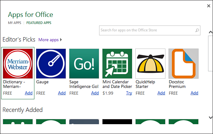
Figure 1.11. Apps for Office can expand the functionality of Excel and provide information from web pages.

3. Click on the desired app and it is installed in Excel. It appears as a task pane on the right side of the Excel window or as a floating window on the sheet, as shown in Figure 1.12.

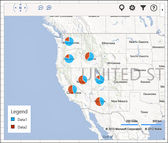
Figure 1.12. An app can be a floating window that charts your data to a map (Bing Maps shown).

4. To see your installed apps, return to the Apps for Office dialog box and click on My Apps in the upper-left corner of the dialog box. You will see all the apps from the store that you own.

5. Select an app from the list and click Insert to open the app in Excel.