7. Sorting Data

This chapter shows you the various ways you can sort your data, even by color. Sorting data is a significant capability in Excel, allowing you to view data from least to greatest, greatest to least, by color, or even by your own customized sort listing.

Preparing Data

Your data should adhere to a few basic formatting guidelines to make the most of Excel’s sorting capabilities:

• There should be no blank rows or columns. The occasional blank cell is acceptable.

• Every column should have a header.

• Headers should be in only one row.

If these guidelines aren’t followed, Excel can get confused and is unable to find the entire table or header row on its own. Also, Excel can only work with one header row—any rows after the first header row get treated like data.

Opening the Sort Dialog Box

The Sort dialog box allows up to 64 sort levels. Through the dialog box, you can sort multiple columns by values, cell color, font color, or by conditional formatting cell icons. The sort order can be ascending, descending, or by a custom list (see the section “Sorting with a Custom Sequence”). If your data has headers, they will be listed in the Sort By drop-down; otherwise, the column headings (A, B, C, etc.) will be used.

There are four ways to access the Sort dialog box:

• On the Home tab, select Editing, Sort & Filter, Custom Sort.

• On the Data tab, select Sort & Filter, Sort.

• Right-click any cell and select Sort, Custom Sort.

• From a filter or Table drop-down, select Sort by Color, Custom Sort.

Sorting by Values

When you use the Sort dialog box, Excel applies each sort in the order it appears in the list. In Figure 7.1, the Region column will be sorted first. The Customer column will be sorted second, as outlined in the following steps:

1. Ensure that the data has no blank rows or columns and that each column has a one-row header.

2. Select a cell in the data. Excel will use this cell to determine the location and size of the data table.

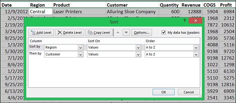
Figure 7.1. Use the Sort dialog box to sort data by multiple levels.

3. Go to Home, Editing, Sort & Filter, Custom Sort to open the Sort dialog box.

4. Make sure the My Data Has Headers check box is selected. Excel will not select the headers themselves, only the data.

5. Make sure all the data’s columns and rows are selected. If they are not all selected, a blank column or row exists, confusing Excel as to the size of your table. Exit from the Sort dialog box, delete the blank columns and rows, and start the process again.

6. From the Sort By drop-down, select the first column header, Region, to sort by.

7. From the Sort On drop-down, select Values.

8. From the Order drop-down, select the order by which the column’s data should be sorted, A to Z.

9. To add another sort column, this time for Customer, click Add Level and repeat steps 6 to 8. Repeat these steps until all the columns to sort by are configured, as shown in Figure 7.1.

10. If you realize that a field is in the wrong position, use the up or down arrows at the top of the dialog box to move the field to the correct location.

11. Click OK to sort the data.

When you look at the data after it is sorted, you’ll notice the regions are grouped together; for example, Central will be at the top of the list. Within Central, the customer names will be alphabetized. If you scroll down to the next region, East, the customer names will be alphabetized within that region. If the data should have listed the customers and then the regions, the two sort fields need to be switched so that Excel sorts the Customer field first and the Region field second.

Sorting by Color or Icon

Although sorting by values is the most typical use of sorting, Excel can also sort data by fill color, font color, or an icon set from conditional formatting. You can apply fill and font colors through conditional formatting or the cell format icons.

In addition to sorting colors and icons through the Sort dialog box, the following options are also available when you right-click a cell and select Sort from the context menu:

• Put Selected Cell Color on Top

• Put Selected Font Color on Top

• Put Selected Cell Icon on Top

If you use one of the preceding options to sort more than one color or icon, the most recent selection is placed above the previous selection. So, if yellow rows should be placed before the red rows, sort the red rows first, and then sort the yellow rows.

In Figure 7.2, conditional formatting was used to highlight in red the top 10 profit record, and yellow was used to highlight the ones in the bottom 10%. The data was then sorted using the following steps so that the red cells are at the top and the yellow directly beneath:

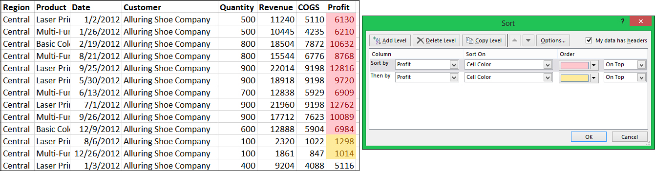
Figure 7.2. You can use the Sort dialog box to sort cells by more than just their values, such as the cell color.

1. Ensure that the data has no blank rows or columns and that each column has a one-row header.

2. Select a cell in the data. Excel will use this cell to determine the location and size of the data and highlight what it sees as the data table.

3. Right-click the cell and select Sort, Custom Sort.

4. Make sure the My Data Has Headers check box in the upper-right corner is selected. Excel will not select the headers themselves.

5. Make sure all the data’s columns are selected. If they are not all selected, a blank column exists, confusing Excel as to the size of your table.

6. From the Sort By drop-down, select the first column header to sort by, Profit.

7. From the Sort On drop-down, select Cell Color.

8. From the first Order drop-down, select the color by which the column’s data should be sorted.

9. From the second Order drop-down, select whether the color should be sorted to the top or bottom of the data. If you select multiple colors to sort at the top of the data, the colors will still appear in the order chosen.

10. Click Add Level to include the yellow Profit cells in the sort and repeat steps 6 to 9. Repeat these steps until all the columns to sort by are configured.

11. If you realize a field is in the wrong order, use the up or down arrows to move it to the correct location.

12. Click OK to sort the data.

Using the Quick Sort Buttons

The quick sort buttons offer one-click access to sorting cell values. They do not work with colors or icons. There are four ways to get to the quick sort buttons:

• On the Home tab, select Editing, Sort & Filter, Sort A to Z¹ or Sort Z to A¹.

• On the Data tab, select Sort & Filter, AZ or ZA.

• Right-click any cell and select Sort, Sort A to Z¹, or Sort Z to A¹.

• From a filter drop-down, select Sort A to Z¹ or Sort Z to A¹.

¹The actual button text may change depending on the type of data in the cell. For example, if the column contains values, the text will be Sort Smallest to Largest. If the column contains text, it will be Sort A to Z.

The quick sort buttons are very useful when sorting a single column. When sorting just one column, make sure you select just one cell in the column. If you select more than one cell, Excel sorts the selection, not the column. It prompts to verify that this is the action you want taken before doing it. Also ensure there are no adjacent columns or Excel will want to include them in the sort. If there are adjacent columns, select the entire column before sorting.

If you use the quick sort buttons to sort a table of more than one column, Excel sorts the entire table automatically. Because there is no dialog box, it’s very important that every column have a header. If just one header is missing, Excel will not treat the header row as such and will include it in the sorted data.

Quick Sorting Multiple Columns

If you keep in mind that Excel keeps previously organized columns in order as new columns are sorted, you can use this to sort multiple columns. For example, if the Customer column is organized, Excel doesn’t randomize the data in that column when the Region column is sorted. Instead, Customer retains its order to the degree it falls within the Region sort. The trick is to apply the sorts in reverse to how they would be set up in the Sort dialog box.

To manually perform the “Sort by Values” example shown in Figure 7.2, follow these steps:

1. Make sure all columns have headers. If even one column header is missing, Excel will not sort the data properly.

2. Select a cell in the column that should be sorted last, the Customer column.

3. Click the desired quick sort button on Data, Sort & Filter.

4. Select a cell in the next column, Region, to be sorted.

5. Click the desired quick sort button on Data, Sort & Filter.

6. The table is now sorted by Region and then Customers within each region.

Randomly Sorting Data

Excel doesn’t have a built-in tool to do a random sort, but by using the RAND function in a column by the data and then sorting, you can create your own randomizer. For example, you have your alphabetical list of students ready to give their project presentations. Instead of going in alphabetical order, you can randomize the list by following these steps:

1. Add a new column to the right of the data. Give the column a header, such as Random.

2. In the first cell of the new column, type =RAND() and press Ctrl+Enter (this keeps the formula cell as the active cell). The formula will calculate a value between 0 and 1.

3. Double-click the fill handle in the lower-right corner of the cell to copy the formula to the rest of the rows in the column.

4. Select one cell in the new column.

5. Go to Home, Editing, Sort & Filter, AZ. The list will be sorted in a random sequence, as shown in Figure 7.3.

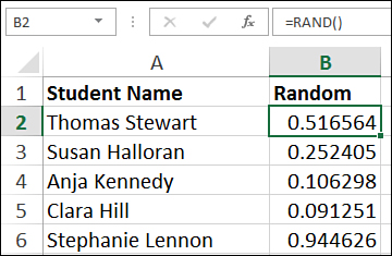
Figure 7.3. Randomly sort the list of students with the RAND function instead of using the expected alphabetical order.

6. Delete the data in the temporary column that you added in step 1.

Sorting with a Custom Sequence

At times, data might need to be sorted in a custom sequence that is neither alphabetical nor numerical. For example, you might want to sort by month, by weekday, or by some custom sequence of your own. You can do this by sorting by a custom list.

Within the Sort dialog box, you can select Custom List from the Order field for each level of sort configured. When this option is selected, the Custom Lists dialog box opens, from which you can select the custom list to sort the selected column by.

The data table in Figure 7.4 has three types of printers: Basic ColorJet, Laser, and Multi-Function. You need to sort the data by Laser, ColorJet, then Multi-Function, but that isn’t alphabetical or reverse alphabetical. To do this sort, first create a custom list with the exact text used in the table. Then, you can sort the table by your custom list. To create a custom list and sort your data by it, follow these steps:

1. Ensure that the data has no blank rows or columns and that each column has a one-row header.

2. Select a cell in the data. Excel will use this cell to determine the location and size of the data.

3. Go to Home, Editing, Sort & Filter, Custom Sort to open the Sort dialog box.

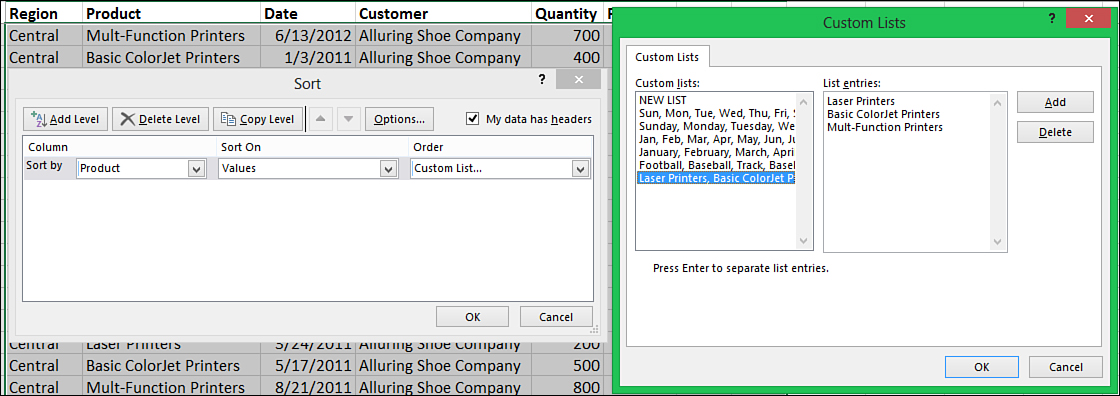
Figure 7.4. Data can be sorted by a custom list, such as a specific order of products.

4. Make sure the My Data Has Headers check box in the upper-right corner is selected. Excel will not select the headers themselves.

5. Make sure all the columns and rows are selected. If they are not all selected, a blank column or row exists, confusing Excel as to the size of your data. Exit from the Sort dialog box, remove the blank column or rows, and then return to the Sort dialog box.

6. From the Sort By drop-down, select the column header, Product, to sort by.

7. From the Sort On drop-down, select Values.

8. From the Order drop-down, select Custom List. The Custom Lists dialog box, shown in Figure 7.4, appears.

9. The list box on the left provides a list of available custom lists. Selecting one will display all the entries in the right list box. Select the desired list and click OK.

10. If you need to sort by other columns, click Add Level. Otherwise, skip to step 13.

11. Repeat steps 6 to 8. If you don’t need to use another custom list, select the desired order from the drop-down instead of Custom List.

12. If you realize that a field is in the wrong order, use the up or down arrows to move it to the correct location.

13. Click OK to sort the data.

Rearranging Columns Using the Sort Dialog Box

If you receive a report where you always have to rearrange the columns to suit yourself, you can use the option of sorting from left to right instead of from top to bottom. To create a custom sort order and then sort your data according to it, follow these steps:

1. Insert a new blank row above the headers.

2. In the new row, type numbers corresponding to the new sequence of the columns, with 1 being the leftmost column, then 2, 3, and so on, until each column has a number denoting its new location.

3. Select a cell in the data range.

4. Press Ctrl+* (or Ctrl+Shift+8) to select the current region, including the two header rows.

5. Go to Home, Editing, Sort & Filter, Custom Sort to open the Sort dialog box.

6. Click the Options button to open the Sort Options dialog box.

7. Select Sort Left to Right.

8. Click OK to return to the Sort dialog box.

9. In the Sort By drop-down, select the row in which the numbers you added in step 2 are located.

10. In the Order drop-down, make sure Smallest to Largest is selected.

11. Click OK and Excel will rearrange the columns.

12. Delete the temporary row added in step 1.

Rearranging Columns Using the Mouse

If you have just a few columns to rearrange, you can use a combination of keyboard shortcuts and the mouse to rearrange them quickly. To quickly move a column to a new position, follow these steps:

1. Select a cell in the column to move.

2. Press Ctrl+Spacebar to select the entire column.

3. Place the cursor on the dark border surrounding the selection, hold down the right mouse button, and drag the column to the new location.

4. When you release the mouse button, a context menu appears, as shown in Figure 7.5. Select Shift Right and Move.

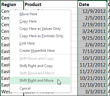
Figure 7.5. Use Shift Right and Move to quickly move a column to a new location.

5. The data will rearrange itself, inserting the column in the new location and moving other columns over to the right to make room.

Fixing Sort Problems

If it looks like the data did not sort properly, refer to the following list of possibilities:

• Make sure no hidden rows or columns exist.

• Use a single row for headers. If you need a multiline header, either wrap the text in the cell or use Alt+Enter to force line breaks in the cell.

• If the headers were sorted into the data, there was probably at least one column without a header.

• Column data should be of the same type. This might not be obvious in a column of ZIP Codes where some, such as 57057 are numbers, but others that start with 0s are actually text. To solve this problem, convert the entire column to text.

• If sorting by a column containing a formula, Excel will recalculate the column after the sort. If the values change after the recalculation, such as with RAND, it may appear that the sort did not work properly, but it did.