
Chapter 3 Manage Storage
Managing storage and performing data maintenance on a regular schedule is a critical aspect of ensuring proper performance and availability of SQL Server, both on-premises and in the cloud. A comprehensive understanding of the concepts and technologies is necessary to a successfully running SQL Server environment, and thoughtful and appropriate care must be taken to ensure an appropriate SLA is achieved.
Skills in this chapter:
Skill 3.1: Manage SQL Storage
Skill 3.2: Perform database maintenance
Skill 3.1: Manage SQL Storage
Storage is one of the key performance and availability aspects of SQL Server regardless of the size of the instance and environment, and this applies to both on-premises as well as the cloud. At the rate that server processing power is increasing, storage can easily become a bottleneck. These bottlenecks can be avoided with proper understanding of how SQL Server uses storage, and this skill looks at the different storage options for SQL Server and how to properly manage them for performance and availability.
This skill covers how to:
Manage SMB file shares
The SMB (Server Message Block) protocol is a network file sharing protocol that provides the ability to access files or resources on a remote server or file share and read/write to files on a network computer. For SQL Server, this means that SQL Server can store use database files on SMB file shares starting with SQL Server 2008 R2. Starting with SQL Server 2008 R2, support for SMB supports SMB for stand-alone SQL Servers, but later releases of SQL Server support SMB for clustered SQL Servers and system databases.
Windows Server 2012 introduced version 3.0 of the SMB protocol, which included significant performance optimizations. One of those optimizations included improvements for small random read/write I/O operations, which is idea for SQL Server. Another optimization is that it turns on MTU (Maximum Transmission Units), which significantly increases performance for large sequential transfers that SQL Server can again take advantage of with SQL Server data warehouse and backup/restore operations.
The addition of the SMB 3.0 protocol in Windows Server 2012 also includes a few performance and availability improvements, such as:
SMB Scale Out Administrators can create file shares that provide concurrent direct access to data files on all nodes in a file server cluster using Cluster Shared Volumes, allowing for improved load balancing and network bandwidth.
SMB Transport Failover Clients can transparently reconnect to another cluster node without interrupting applications writing data to the file shares.
SMB Direct Provides high performance network transport via network adapters that use Remote Direct Memory Access (RDMA). For SQL Server, this enables a remote file server to resemble local storage.
SMB Multichannel Enables server applications to take advantage of all available network bandwidth as well as be resilient to a network failure through the aggregation of network bandwidth and fault tolerance capabilities.
With the improvements to the SMB protocol, this means that SQL Server environments running on Windows Server 2012 or higher (and with SQL Server 2012 or higher) can now place their system database and create user database data files placed on the SMB file shares, knowing it is backed by network performance and integrity.
In order for SQL Server to use the SMB file shares, the SQL Server needs to have the FULL CONTROL permissions and NTFS permissions on the file SMB file share folders. The best practice is that you use a domain account as the SQL Server services account, otherwise you simply need to grant the appropriate permission to the share folder.
To use an SMB file share in SQL Server, simply specify the file path in the form of a UNC path format, such as \ServerNameShareName or \ServerNameShareName. Again, you need to be using SQL Server 2012 or higher, and the SQL Server service and the SQL Agent service accounts need to have FULL CONTROL and NTFS share permissions.
To create a database on an SMB share you can use SQL Server Management Studio or T-SQL. As shown in Figure 3-1, in the New Database dialog box, the primary data file and log file is placed on the default path, and a secondary file is specified with a UNC path to an SMB share.

Figure 3-1 Creating a database with a secondary data file on an SMB file share
There are a few limitations when using SMB file shares, including the following, which is not supported:
Mapped network drives
Incorrect UNC path formats, such as \...z$, or \localhost...
Admin shares, such as \serernameF$
Likewise, this can be done in Azure using Azure Files, which create SMB 3.0 protocol file shares. The following example uses an Azure Virtual Machine running SQL Server 2016 and an Azure storage account, both of which have already been created. Another section in this chapter discusses Azure storage and walks through creating a storage account.
Once the storage account has been created, open it up in the Azure portal and click the Overview option, which shows the Overview pane, shown in Figure 3-2.

Figure 3-2 Azure storage services
The Overview pane shows the available storage services, one of which is the Files service, as shown and highlighted in Figure 3-2. More about this service is discussed later in this chapter. Clicking the File service opens the File service pane, shown in Figure 3-3.

Figure 3-3 The File Service pane
The File Service pane shows details about the file service and any file shares that have been created. In this case, no files shares have been created so the list is empty. Therefore, click the + File Share button on the top toolbar to create a new file share, which opens the New File Share pane, shown in Figure 3-4.
Creating a new file share is as simple as providing a file share name and the disk size quota. The quota is specified in GB with a value up to 5120 GB, and in this example a value of 100 GB was specified. Click OK when done, which takes you back to the File Service blade that now displays the newly created file share.
Once the file shares are created they can be mounted in Windows and Windows Server, both in an Azure VM as well as on-premises. They can be mounted using the Windows File Explorer UI, PowerShell, or via the Command Prompt.
When mounting the drive, the operating system must support the SMB 3.0 protocol, and most recent operating systems do. Windows 7 and Windows Server 2008 R2 support SMB 2.1, but both Windows Server 2012 and higher, as well as Windows 8.1 and higher, all include SMB 3.0, although Windows Server 2012 R2 as well as Server Core contain version 3.2, as does Windows Server 2016.

Figure 3-4 Configuring a new file share
As previously mentioned, Azure file shares can be mounted in Windows using the Windows File Explorer UI, PowerShell, or via the Command Prompt. Regardless of the option, the Storage Account Name and the Storage Account Key are needed. Additionally, the SMB protocol communicates over TCP port 445, and you need to ensure your firewall is not blocking that port.
The storage account name and key can be obtained from the Access keys option in your Azure storage account. For the storage key, either the primary or secondary key will work.
Probably the easiest way to mount the drive is by using the Windows Command Prompt and the Net Use command and specifying the drive letter, account name, and account key, as shown in the code below. To execute, replace the <account name> with the name of your storage account name, and replace the <storage account key> with the primary key for the storage account.
net use Z: \< account name>.file.core.windows.netdatadisk1 /u:AZURE<account name>
<storage account key>
Figure 3-5 shows the execution of the Net Use command to mount the SMB file share as drive Z, specifying the account name and account key. You will get an error if port 445 is not open on your firewall. Some ISPs block port 445 so you will need to check with your provider.
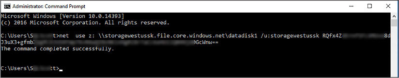
Figure 3-5 Mounting the new file share with command prompt
Once the file share is mounted, you can view the new mounted drive in Windows Explorer as a Network location, as shown in Figure 3-6.

Figure 3-6 The new file share in Windows Explorer
With the new SMB file share mounted and ready to use, files and folders can be created on it, including SQL Server data files. For this example, a folder on the file share called Data is created to add SQL Server secondary data files.
Figure 3-7 shows how to create a new database on-premises with a data file on a SMB file share. When creating a new database in SQL Server Management Studio, in the New Database dialog box, the primary data file and log file are placed on the default path, and a secondary file is specified with a UNC path to the Azure file share.

Figure 3-7 Creating a database with a secondary data file on an Azure File share with SMB
Similar to on-premises SMB file shares, the same permissions and security requirements apply when using Azure Files. The SQL Server services still needs FULL CONTROL permissions to the share, as well as NTFS. Once this is configured, you are able to create databases using SMB file shares.
It used to be that using file shares as a storage option for data files was unthinkable. The risks were too high; file shares were too slow causing performance issues, data integrity was an issue, and the SMB protocol was not kind to the likes of applications such as SQL Server, which had rigorous I/O workloads.
However, this changed with the release of version 3.0 of the SMB protocol, which addresses these issues by implementing the features and capabilities discussed earlier, allowing SQL Server to be a prime target for using SMB file shares.
Manage stretch databases
Stretch Database is a feature added to SQL Server 2016 with the goal of providing cost efficient storage for your cold data. Hot data refers to data that is frequently accessed on fast storage, warm data is data that is less-frequently accessed data preferably stored on less-performant storage, and cold data refers to rarely accessed data that is hopefully stored on slow storage.
In the SQL Server environment, hot, warm, and cold data is typically stored on the same storage devices for easy access, even though cold data is, as mentioned, rarely accessed. The result of storing cold data causes the database to fill up with unused data, and increases storage costs as the hot/warm data becomes cold data.
Stretch Database aims to address these issues by allowing you to dynamically “stretch” cold transactional data to the cloud where storage is less expensive thus freeing up disk space locally. There are several benefits to using Stretch Database:
Low cost By moving cold data from on-premises to the cloud, storage costs can be up to 40 percent less.
No application changes Even though data is moved to the cloud, there are no application change requirements to access the data.
Security Existing security features such as Always Encrypted and Row-Level Security (RLS) can still be implemented.
Data maintenance On-premises database maintenance, including backups, can now be done faster and easier.
One of the main keys to understand with Stretch Database is the second bullet point; no application changes are required. How does this work? When a table is “stretched” to Azure and the cold data moved into Azure SQL Database, the application still sees the table as a single table, letting SQL Server manage the data processing.
For example, let’s say you have an Orders table with orders that date back five years or more. When stretching the Orders table, you specify a filter that specifies what data you want moved to Azure. When querying the Orders table, SQL Server knows which data is on-premises and which has been moved to the cloud, and handles the retrieval of data for you. Even if you execute a SELECT * FROM Orders statement, it retrieves the data from on-premises as well as retrieves the data from Azure, aggregates the results, and returns the data. Thus, there is no need to change the application.
Understand, though, that there is some latency when querying cold data. The latency depends really on how much data you are querying. If you are querying very little, the latency is very small. If you are executing SELECT *, you might need to wait a bit more. Thus, the amount of data you determine as “cold” should be an educated decision.
Another key point is that Stretch Database allows you to store your cold data in Azure SQL Database, which is always online and available, thus providing a much more robust retention period for the cold data. And, with the cold data stored in Azure SQL Database, Azure also manages the storage in a high-performance, reliable, and secure database.
Stretch Database must be enabled at the instance level prior to enabling Stretch at the database or table level. Enabling Stretch Database at the instance level is done by setting the remote data archive advanced SQL Server option via sp_configure.
EXEC sp_configure 'remote data archive, '1';
GO
RECONFIGURE
GO
At the database level, enabling Stretch Database can be done one of two ways; through T-SQL or through the Stretch Database Wizard, and Stretch must be enabled at the database level before stretching a table. The easiest way to enable stretch at the database level is through the Stretch Database Wizard within SQL Server Management Studio. You can either right mouse click the database for which you want to enable Stretch (Tasks > Stretch > Enable), or right mouse click the specific table you want to stretch (Stretch > Enable), as shown in Figure 3-8.
Either option starts the Stretch Database Wizard and enables stretch, the only difference being that right-clicking on the table will automatically select the table in the Wizard, whereas right-clicking on the database will not select any tables and asks you which tables to stretch.

Figure 3-8 Launching the Stretch Database Wizard
The first page of the Stretch Wizard is the Introduction page, which provides important information as to what you need in order to complete the wizard. Click Next on this page of the wizard, and then the Select Tables page appears, shown in Figure 3-9.
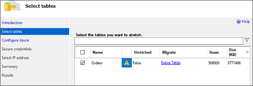
Figure 3-9 Selecting the tables to stretch to Azure
In the Select Tables page, select the tables you want to stretch to Azure by checking the check box. Each row in the list of tables specifies whether the tables has been stretched, how much of the table has been stretched, how many rows are currently in the table, and the approximate size of the data.
Figure 3-9 shows that the Orders table has not been stretched, and that the entire table, all 50,000 rows, will be stretched to Azure. A warning is also given, so let’s address the warning first. The structure of the Orders table looks like this:
CREATE TABLE [dbo].[Orders](
[OrderID] [int] IDENTITY(1,1) NOT NULL,
[CustomerID] [int] NOT NULL,
[SalespersonPersonID] [int] NOT NULL,
[PickedByPersonID] [int] NULL,
[ContactPersonID] [int] NOT NULL,
[BackorderOrderID] [int] NULL,
[OrderDate] [date] NOT NULL,
[ExpectedDeliveryDate] [date] NOT NULL,
[CustomerPurchaseOrderNumber] [nvarchar](20) NULL,
[IsUndersupplyBackordered] [bit] NOT NULL,
[Comments] [nvarchar](max) NULL,
[DeliveryInstructions] [nvarchar](max) NULL,
[InternalComments] [nvarchar](max) NULL,
[PickingCompletedWhen] [datetime2](7) NULL,
[LastEditedBy] [int] NOT NULL,
[LastEditedWhen] [datetime2](7) NOT NULL,
CONSTRAINT [PK_Sales_Orders] PRIMARY KEY CLUSTERED
(
[OrderID] ASC
) ON [PRIMARY]
) ON [PRIMARY] TEXTIMAGE_ON [PRIMARY]
GO
Not very exciting, but the thing to point out is that the Orders table does contain a Primary Key on the OrderID column. The warning is therefore informing you that primary keys or unique keys are only enforced on the rows in the local table and not on the table in Azure. Fair enough, so we can move on from that.
The next item of importance is the Migrate column. By default, all the rows of a selected table, the entire table, are set to be migrated to Azure. This is not what we want, recalling from the earlier hot data/cold data discussion. The goal with Stretch Database is to migrate only cold data to Azure; things like closed orders, or orders passed a certain data (order history), for example.
To fix this, click the Entire Table link, which opens the dialog shown in Figure 3-10. This dialog allows you to apply a filter to specify which rows are to be migrated to Azure. To do this, select the Choose Rows option, and then provide a name for the filter function. This function does not need to already exists. Next, define the WHERE clause filter by picking a column from the table on which to filter, specifying the operator, and then providing a value.

Figure 3-10 Configuring the rows to migrate to zure
In this example, the OrderDate column is being used as the filter for the WHERE clause, specifying that any order older than January 1, 2017 should be migrated to Azure. To test the query, click the Check button, which checks the function by running a sample query that is displayed in the text box below the filter. This text box is read only and not editable. It is for display purposes only. If the sample query returns rows, the test is reported as successful and you can click Close.
The Migrate column back, the Select tables page of the wizard now shows the name of the function it will use to migrate the data to Azure, as shown in Figure 3-11.

Figure 3-11 Configured Select Tables page of the Stretch Database Wizard
Click Next to continue with the wizard, which shows the Configure Azure page, shown in Figure 3-12. The Configure Azure page is where you specify the region in which to either create a new Azure SQL server or select an existing one and in which region, and then supply the credentials for the new or existing server.

Figure 3-12 Selecting and configuring the Azure server
The wizard asks you to sign in to your Azure account in order to access the necessary information, such as existing servers if you have selected that option, such as this example. Once the Configure Azure page is configured, click Next, which displays the Secure credentials page, shown in Figure 3-13.

Figure 3-13 Providing a database master key password
Enter, and confirm, a password on the Confirm Credentials page. As part of the Stretch migration, the wizard creates a database master key. This key is used to secure the credentials that Stretch Database uses to connect to the remote database in Azure.
If the wizard detects an existing database master key, it only prompts you for the existing password. Otherwise it creates a new key and the wizard prompts you to enter and confirm a password. Click Next to move to the Select IP address page of the wizard, shown in figure 3-14.

Figure 3-14 Providing the IP address for the database-level firewall rule
As reviewed in Chapter 2, access to an Azure SQL Database is restricted to a set of known IP addresses through a set of firewall rules. Firewall rules grant access to a database or databases based on the originating IP address of each request. As such, the Select IP Address page of the wizard provides the option to use the public IP address of your SQL Server, or a manually specified IP address range. The recommended option is to manually specify the IP address. The wizard creates the appropriate database-level firewall rule in Azure to allow SQL Server to communicate with the SQL Database in Azure.
Click Next to go to the Summary page, review the details, and then click Next to begin the migration and view the Results page, shown in Figure 3-15.

Figure 3-15 Completed Stretch Database migration
As you can see in Figure 3-15, there are quite a number of steps. The target database was created on the specified Azure SQL server, the database master key created, the firewall rule created, the function created on the local SQL Server, and then the migration began.
What is interesting to note is that this wizard completed before the migration was 100 percent complete; you’ll see that shortly. However, the key point is that Stretch was configured on both ends, on-premises and the cloud, and the migration kicked off. To verify the migration process, connect to the Azure SQL server in SQL Server Management Studio and expand the databases node, wherein you see a Stretch Database-named Orders table, as shown in Figure 3-16.

Figure 3-16 Stretched table in Azure within SQL Server Management Studio
The stretched Orders table is like any other database. By default, a Standard-tier SQL Database is created, but you can change the service tier to get better performance if you plan on querying the data frequently. However, querying the data frequently sort of defeats the purpose of Stretch Database and cold storage. Thus, you need to decide what the appropriate performance level you need is, and if the default is too much or too little. Service tiers are discussed later in this chapter.
However, because it is a normal database, you can connect to it via SQL Server Management Studio and query the data and see how much data is in there. Because the Stretch Wizard completed prior to 100 percent data migration (which is by design), the data is migrated to Azure over a period of time. Depending on how much data is being migrated, the migration process could be quick, or it could take a while.
There is a better way to see what is going on with the Stretch environment, including the number of rows in each table, the status, and troubleshoot each stretch-enabled database. The Stretch Database Monitor is built into SQL Server Management Studio, and you can get to it by right-clicking the database that has been stretched, and selecting Tasks -> Stretch -> Monitor from the context menu, as shown in Figure 3-17.

Figure 3-17 Opening the Stretch Database monitor
The Stretch Database Monitor, shown in Figure 3-18, has two sections. The upper section of the page displays general information both of the on-premises SQL Server and the remote Azure SQL database. The lower portion of the monitor page displays the status data migration for each stretch-enabled table in the database.

Figure 3-18 The Stretch Database Monitor
The monitor page refreshes every 60 seconds, thus if you watch the monitor page long enough you see the Local Rows number decrease and the Rows In Azure number increase, until all the rows that match the filter criteria have been migrated to Azure.
Stretch Database can be disabled either through SQL Server Management Studio or via T-SQL. There are two options when disabling stretch, bringing the data in Azure back to on-premises, or leaving the data in Azure. Leaving the data in Azure abandons the remote data and disables stretch completely. In this scenario, you have data in two locations but not stretched environment. Meaning, you now have to execute a second query to access the cold data.
Bringing the data back to on-premises copies, not moves, the data from Azure back to on-premises and disables stretch. Again, you now have data in two locations, but in this case, you have the same data in two locations. In addition, this option incurs data transfer costs because now you have data leaving the data center.
You should gather from these two scenarios that disabling stretch does not delete the remote table or database in Azure. Thus, if you want to permanently disable stretch for a table, you need to manually delete the remote table.
To disable Stretch, right-click the table you want to stop stretching and select Stretch -> Disable, then select the appropriate option. The Recover Data And Disable Stretch dialog, shown in figure 3-19, shows that Stretch has been disabled successfully.

Figure 3-19 Disabling Stretch Database
However, if you selected the option to bring data back from Azure, the migration of data back to on-premises is so the actual disabling of Stretch might take a bit depending on how much data is in Azure.
It was mentioned earlier about the difference between hot, warm, and cold data, with cold data typically stored on a slower storage option. One of the great things about Stretch Database is that as a storage option, part of managing Stretch Database is selecting the performance level of the remote storage, which in this case, is an Azure SQL database. The different service tiers and performance levels are discussed later in this chapter.
Identifying databases and tables for Stretch Database
One of the main goals of Stretch Database is to provide cost efficient storage for your cold data. The question then becomes how to identify tables that would make good Stretch Database candidates. While there is no hard, fast rule, the general rule of thumb is any transactional table with large amounts of cold data. For example, the table used in this chapter contains an OrderDate column, and stored orders that date back many years. This example simply says “any order with an order date older than 1/1/2017” is considered cold data. Another approach would have been to include an OrderStatus column, with values of “open,” “closed,” “Pending,” and so on. In this situation we could have defined the filter as any order with an order status of “closed” as cold and migrated to Azure.
Any “history” table is a good candidate for stretch. SQL Server also introduced a feature called Temporal tables, which is a system-versioned temporal table designed to keep a full history of data changes for each point-in-time analysis. These tables are excellent candidates for stretch as you can migrate all or part of the associated history to Azure.
Stretch Database limitations
Stretch Database does have a few limitations that prevents a table from being stretched. They are:
Tables
Tables that have more than 1,023 columns or 998 indexes
FileTables or tables that contain FILESTREAM data
Replicated tables, or tables that use Change Tracking or Change Data Capture
Memory-optimized tables
Indexes
Full text
XML
Spatial
Indexed Views
Data types
sql_variant
XML
CLR
Text, ntext, image
timestamp
Computed columns
Constraints
Default constraints
Foreign key constraints that reference the table
Likewise, remote tables have limitations. As reviewed earlier, stretch-enabled tables do not enforce primary keys or unique constraints. You also cannot update or delete rows that have been migrated, or rows that are eligible for migration.
Configure Azure storage
Azure storage is a managed service providing enterprise-ready storage capabilities. Azure storage is comprised of three storage services; Blob, File, and Queue. Until recently, Table storage was also a part of Azure storage, but Azure Table storage is now part of Azure Cosmos DB.
The goal with Azure storage is to provide an array of storage options that are highly available, scalable, secure, and redundant. Azure storage provides this by implementing an architecture that allows for the storage and access of immense amounts of data. Figure 3-20 shows the Azure storage architecture at a high level.

Figure 3-20 Windows Azure Storage architecture
As shown in Figure 3-20, Azure storage consists of several components:
Storage Stamps A cluster of N racks of storage nodes, each rack is built out as a separate fault domain. Clusters range from 10 to 20 racks.
Stream Layer Stores the bits on disk and is responsible for distributing and replicating the data across multiple servers for data durability with the stamp.
Partition Layer Provides scalability by partitioning data within the stamp. Also provides transaction ordering and caching data to reduce disk I/O.
Front-Ends Comprised of a number of stateless servers, is responsible for handling incoming requests. Is also responsible for authenticating and authorizing the request.
Location Service Manages all of the storage stamps, and the account namespace across the stamps. This layer also allocates accounts to storage stamps and manages them across the stamp for disaster recovery and load balancing.
The Location Service tracks and manages the resources used by each storage stamp. When a request for a new storage request comes in, that request contains the location (region) in which to create the account. Based on this information, the Location Service selects the storage stamp within that location best equipped to handle the account and selects that stamp as the primary stamp (based on load across stamps and other criteria).
The Location Service stores the account metadata in the selected stamp, informing the stamp that it is ready to receive requests for that account. The Location Service then updates the DNS, allowing incoming requests to be routed from that account name to that storage stamps VIP (Virtual IP). The VIP is an IP address that the storage stamp exposes for external traffic.
Thus, to use any of the storage services of Azure Storage you must first create an Azure Storage account. Azure Storage accounts can be created using the Azure portal, or by using PowerShell or the Azure CLI.
The New-AzureRmStorageAccount PowerShell cmdlet is used to create a general-purpose storage account that can be used across all the services. For example, it can be used as shown in the code snippet below. Be sure to replace <storageaccountname> and <resourcegroupname> with a valid and available storage account name and resource group in your subscription.
New-AzureRmStorageAccount
-ResourceGroupName "<resourcegroupname>"
-Name "<storageaccountname>"
-Location "West US"
-SkuName Standard_LRS
-Kind Storage -EnableEncryptionService Blob
The Azure CLI is similar (replacing <storageaccountname> and <resourcegroupname> with a valid and available storage account name and resource group in your subscription):
az storage account create --name <storageaccountname> --resource-group <resourcegroupname> --location eastus --sku Standard_LRS --encryption blob
Both PowerShell and the Azure CLI can be executed directly from within the Azure Portal. However, this example shows how to create the Storage account in the Azure portal. Within the portal, select New -> Storage, and then select the Storage account option, which opens the Create Storage Account blade, shown in Figure 3-21.

Figure 3-21 Creating and configuring an Azure storage account
Configuring Azure storage appropriately is important because there are several options, which can help with performance and availability.
Name The name of the storage account. Must be unique across all existing account names in Azure, and be 3 to 24 characters in length of lowercase letters and numbers.
Deployment Model Use Resource Manager for all new accounts and latest Azure features. Use Classic if you have existing applications in a Classic virtual network.
Account Kind General purpose account provides storage services for blob, files, tables, and queues in a unified account. The other account option, Blob Storage, are specialized for storing blob data.
Performance Standard accounts are backed by magnetic drives and provide the lower cost per GB, and are best used where data is accessed infrequently. Premium storage is backed by SSD (solid state drives) and provide consistent, low-latency performance. Premium storage can only be used with Azure virtual machine disks for I/O intensive applications.
Replication Data in Azure storage is always replicated to ensure durability and high availability. This option selects the type of replication strategy.
Secure Transfer Required When enabled, only allows requests to the storage account via secure connections.
When selecting the Blob Storage Account kind, the additional configuration option of the Access tier is available, with the options of choosing Cool or Hot, which specifies the access pattern for the data, or how frequently the data is accessed.
The Virtual network option is in Preview; thus, it is left disabled for this example. However, this configuration setting grants exclusive access to the storage account from the specified virtual network and subnets.
It should be noted that the Performance and Replication configuration settings cannot be changed once the storage account has been created. As mentioned, unless you are using storage as virtual machine disks, choosing the Standard option is sufficient.
Focusing the Replication configuration option, there are four replication options:
Locally Redundant Replicates your data three times within the same datacenter in the region in which you created the storage account.
Zone-Redundant Replicates your data asynchronously across datacenters with your region in addition to storing three replicas per local redundant storage.
Geo-Redundant Replicates your data to a secondary region that is at least hundreds of miles away from the primary region.
Read-Access Geo-Redundant Provides read-only access to the data in the secondary location in addition to the replication across regions provided by geo-redundant.
In 2014, Azure released the Resource Manager deployment model, which added the concept of a resource group which is essentially a mechanism for grouping resources that share a common lifecycle. The recommended best practice is to use Resource Manager for all new Azure services.
Once the Create storage account page is configured, click Create. It doesn’t take long for the account to be created, so the storage account properties and overview panes, shown in Figure 3-22, will open.
The Overview pane contains three sections; the top section is the Essentials section that displays information about the storage account, the middle section shows the services in the storage account (Blobs, Files, Tables, and Queues), and the lower section displays a few graphs to monitor what is happening within the storage account, including total requests, amount of outgoing data, and average latency.

Figure 3-22 Azure storage account overview
When the account is created, a set of access keys is generated, a primary and secondary key. Each storage account contains a set of keys, and they can be regenerated if ever compromised. These keys are used to authenticate applications when making requests to the corresponding storage account. These keys should be stored in Azure Key Vault for improved security, and best practice states that the keys be regenerated on a regular basis. Two keys are provided so that you can maintain connections using one key while regenerating the other.
Figure 3-23 shows the Access Keys pane, which shows the two access keys and their corresponding connection strings. When regenerating keys, the corresponding connection strings are also regenerated with the new keys. These keys are used to connect to any of the Azure storage services.

Figure 3-23 Retrieving the Azure storage account keys and connection strings
As shown in Figure 3-22, creating an Azure storage account comes with storages services for Blobs, Files, and Queues. Tables is also listed but it is recommended that the new premium Azure table experience be used through Azure Cosmos DB.
Blobs
The Azure Blob service is aimed at storing large amounts of unstructured data and accessed from anywhere. The types of files that can be stored include text files, images, videos, and documents, as well as others. The Blob service is comprised of the following components:
Storage Account The name of the storage account.
Container Groups a set of blobs. All blobs must be in a container.
Blob A file of any time and size.
Thus, a storage account can have one or more containers, and a container can have one or more blobs. An account can contain an unlimited number of containers, and a container can contain an unlimited number of blobs. Think of the structure much like that of Windows Explorer, a folders and files structure with the operating system representing the account.
Because blobs must be in containers, let’s look at containers first. Back in the Overview pane for the storage account, shown in Figure 3-22, click the Blobs tile, which opens the Blob service pane, shown in Figure 3-24. The Blob service pane displays information about the storage account and blob service and lists any containers that exist within that storage account. In this example, the storage account has recently been created so no containers have been created yet. To create a container, click the + Container button on the top toolbar in the Blob service pane, shown in Figure 3-24, which opens the New Container dialog shown in Figure 3-25.

Figure 3-24 The Azure blob service pane
Adding and configuring a new container is as simple as providing a container name and specifying a public access level, as you can see in Figure 3-25.

Figure 3-25 Adding a new blob service container
Container names must be lower case and begin with a letter or number, and can only contain letters, numbers, and the dash character. Container names must be between three and 63 characters long, and each dash must be immediately preceded by and followed by a letter or number.
As you can see in Figure 3-25, there are three public access level types. The public access level specifies if the data in the container is accessible to the public and how it is accessible.
Private The default value that specifies that the data within the container is available only to the account owner.
Blob Allows public read access for the blobs within the container.
Container Allows public read and list access to the contents of the entire container.
The public access level setting you choose therefore depends on the security requirements of the container and the data within the container. Click OK on the New Container dialog, which returns you to the Blob service pane now showing the newly added container, as shown in Figure 3-26.

Figure 3-26 The blob service pane listing a container
Clicking anywhere on the newly created blob opens the container pane for that particular blob. In Figure 3-27, clicking the Videos container opens the container pane for the Videos container.

Figure 3-27 Listing the contents of the container
The container pane allows you to upload files to the container, delete the container, view the container properties, and more importantly, define access policies. In the container pane, click the Access policy button on the toolbar, which opens the Access policy pane.
The Access policy pane shows defined access policies and if needed, changes the public access level of the container. Leaving the public access level where it is, there should be no policies defined, so click the Add Policy button that opens the Add Policy dialog, shown in Figure 3-28.

Figure 3-28 Defining an access policy on a container
An access policy is defined on a resource, such as in this case, on a container. The policy is used to provide a finer-grained access to the object. When an access policy is applied to a shared access signature (SAS), the shared access signature inherits the constraints of the policy.
For example, in Figure 3-28 the policy is defined with an identifier, with all four permissions selected. The four permissions are Read, Write, Delete, and List. A time limit has also been specified of one month, from 10/1 to 10/31.
A shared access signature provides delegated access to any resource in the storage account without sharing your account keys. This is the point of shared access signatures; it is a secure way to share storage resources without compromising your account keys.
Shared access signatures cannot be created in the Azure portal, but can be created using PowerShell or any of the Azure SDKs including .NET. The idea is that you define the access policy in the portal (as you did in Figure 3-28), and then apply the access policy to a shared access signature to define the level of access.
A few words on blobs before moving on. Azure storage offers three types of blobs:
Block Ideal for storing text or binary files such as documents, videos, or other media files.
Append Similar to block blobs but are optimized for append operations, thus useful for logging scenarios.
Page More efficient for I/O operations, which is why Azure virtual machines use page blogs as operating system and data disks.
Page blobs can be up to 8 TB in size, whereas a single block blob can be made up of up to 50,000 blocks with each block being 100 MB, totaling a bit more than 4.75 TB in total size. A single append block can be made up of up to 50,000 blocks with each block being 4 MB, totaling a little over 195 GB in total size.
Blob naming conventions differ slightly from that of containers, in that a blob name can contain any combination of characters but must be between one and 1024 characters, and are case sensitive.
Files
Azure files provide the ability to create fully managed, cloud-based file shares that are accessible with the industry standard SMB (Server Message Block) protocol. We reviewed the SMB protocol earlier in this chapter, but as a refresher, the SMB protocol is a network sharing protocol implemented in Windows that provides the ability to access files or resources on a remote server or file share and read/write to files on a network computer.
One of the major benefits of Azure files is that the file share can be mounted concurrently both in the cloud as well as on-premises, on Windows, Linux, or macOS. Azure files provide the additional benefit of having additional disk space without the necessity of managing physical servers or other devices and hardware.
Azure File shares are useful when you need to replace, complement, or provide additional storage space to on-premises file servers. Azure file shares can be directly mounted from anywhere in the world, making them highly accessible. Azure Files also enable “lift and shift” scenarios where you want to migrate an on-premises application to the cloud and the application has the requirement of access to a specific folder or file share.
Earlier in this chapter you walked through how to create an Azure File, as seen in Figure 3-4. In the Azure storage overview pane, click the Files tile, which opens the File service pane, shown in Figure 3-29. Earlier you created a file share so that share is listed in the list of file shares.

Figure 3-29 Azure storage file share
Clicking the file share, open the File Share pane, shown in Figure 3-30. Via the File Share pane you can upload files to the share, add directories, delete the share, update the quota, and obtain the connection information for both Windows and Linux by clicking the Connect button.

Figure 3-30 Adding a folder to the Azure file share
In this example, we added a Data directory that was used earlier to add secondary SQL Server data files. Clicking the directory provides the ability to upload files to that directory, add subdirectories, and delete the directory.
The question then becomes one of when to use what service. When do you decide to use Azure blobs, files, or even disks? Use the following points as a guide.
Azure Blobs Your application needs streaming support or has infrequent access scenarios to unstructured data, which needs to be stored and accessed at scale, plus you need access to your data from anywhere.
Azure Files You have a “lift and shift” scenario and you want minimal to no application changes, or you need to replace or complement existing storage.
Azure Disks apply to Azure IaaS virtual machines by allowing you to add additional disk space through the use of Azure storage. To use Azure Disks, you simply need to specify the performance type and the size of disk you need and Azure creates and manages the disks for you.
Change service tiers
Azure SQL Database is a general-purpose, managed relational database in Microsoft Azure that shares its code base with the SQL Server database engine. As a managed service in Azure, the goal is to deliver predictable performance with dynamic scalability and no downtime.
To achieve the predictable performance, each database is isolated from each other with its defined set of resources. These resources are defined in a service tier that are differentiated by a set of SLA options, including storage size, uptime availability, performance, and price, as detailed in Table 3-1.
Table 3-1 Choosing a service tier
Basic |
Standard |
Premium |
Premium RS |
|
Target workload |
Development and Production |
Development and Production |
Development and Production |
*Workloads that can stand data loss |
Max. DB Size |
2GB |
1 TB |
4 TB |
1 TB |
Max DTUs |
5 |
3000 |
4000 |
1000 |
Uptime SLA |
99.99% |
99.99% |
99.99% |
**N/A |
Backup retention |
7 days |
35 days |
35 days |
35 days |
CPU |
Low |
Low, Medium, High |
Medium, High |
Medium |
IO throughput |
Low |
Medium |
Significantly higher than Standard |
Same as Premium |
IO Latency |
Higher than Premium |
Higher than Premium |
Lower than Basic |
Same as Premium |
Columnstore indexing and in-memory OLTP |
N/A |
N/A |
Supported |
Supported |
* Data loss is up to 5 minutes due to service failures
** Not available while Premium RS tier is in preview
Choosing a service tier for our database depends primarily on the storage, uptime, and performance requirements.
DTU
To understand performance in Azure SQL Database is to understand DTUs. DTU, or Database Transaction Unit, is a blended measure of CPU, memory, and I/O. The amount of resources determined per DTU was defined by an OLTP benchmark workload designed and optimized for typical, real-world OLTP workloads. When a performance tier is selected, the DTUs are set aside and dedicated to your database and are not available to any other database, thus the workload of another database does not impact your database or the resources of your database, and likewise your workload does not impact the resources or performance of another database. When your workload exceeds the amount of resources defined by the DTU, your throughput is throttled, resulting in a slower performance and timeouts.
Within each service tier is a set of different performance levels. The following tables (Table 3-2 to Table 3-6) detail the different service tiers and their performance levels.
Table 3-2 Basic Service Tier
Performance Level |
Basic |
Max DTUs |
5 |
Max concurrent logins |
30 |
Max concurrent sessions |
300 |
Table 3-3 Standard Service Tier
Performance Level |
S0 |
S1 |
S2 |
S3 |
Max DTUs |
10 |
20 |
50 |
100 |
Max concurrent logins |
60 |
90 |
120 |
200 |
Max concurrent sessions |
600 |
900 |
1200 |
2400 |
Table 3-4 Continued Standard Service Tier
Performance Level |
S4 |
S6 |
S7 |
S9 |
S12 |
Max DTUs |
200 |
400 |
800 |
1600 |
3000 |
Max concurrent logins |
400 |
800 |
1600 |
3200 |
6000 |
Max concurrent sessions |
4800 |
9600 |
19200 |
30000 |
30000 |
Table 3-5 Premium Service Tier
Performance Level |
P1 |
P2 |
P4 |
P6 |
P11 |
P13 |
Max DTUs |
125 |
250 |
500 |
1000 |
1750 |
4000 |
Max concurrent logins |
200 |
400 |
800 |
1600 |
2400 |
6400 |
Max concurrent sessions |
30000 |
30000 |
30000 |
30000 |
30000 |
30000 |
Table 3-6 Premium RS Service Tier
Performance Level |
PRS1 |
PRS2 |
PRS4 |
PRS6 |
Max DTUs |
125 |
250 |
500 |
1000 |
Max concurrent logins |
200 |
400 |
800 |
1600 |
Max concurrent sessions |
30000 |
30000 |
30000 |
30000 |
The Premium RS service Tier was announced and added in early 2017. It is currently in preview and as such the specifics of the tier may change. The Premium RS service tier was specifically designed for I/O intensive workloads that need the premium performance but do not require the highest availability guarantees.
It helps to understand the relative amount of resources between the different performance level and service tiers, and the impact they have on the database performance. The math is quite easy, in that, changing a service tier for a database from a Premium P1 to a Premium P2 doubles the DTUs and increases the performance level of the database by doubling the amount of resources to the database.
As such, as you begin to gain insight into the performance implications a specific service tier has for your database, you should begin to understand the proper service tier your specific database needs and the potential affect that will take place, either positive or negative, as you change between service tiers.
Based on the above information, it should be obvious that you can change service tiers for your database at any time. Setting the initial performance level at database creation time is a good baseline, but workload demand dictates the proper service tier and performance level for your database and thus you can change it as needed.
In fact, a standard practice is to scale the database up during normal business operating hours, and then scale it down during off hours, saving costs dramatically. Changing service tiers has minimal downtime, typically only a few seconds. Thus, scaling a database should be done at proper times when it does not affect users.
Changing a service tier can be done via several methods, including via the Azure portal, T-SQL, and PowerShell. In the Azure portal, select the database for which you want to change the service tier, and in the Overview pane, select the Pricing tier option, as shown in Figure 3-31.

Figure 3-31 Configuting the pricing tier for a database
The Configure Performance pane opens, shown in Figure 3-32, which opens showing the current service tier for the database. The top section of the Configure Performance displays the different service tiers via four tabs. The tabs contain a description of the service tier and a start cost for the minimum performance level of that service tier.
In this example, the current service tier is Basic with a maximum storage of 2 GB. Using the slider, we can scale the storage from a maximum of 2 GB to a minimum of 100 MB. For the DTU, the only option is 5 for the Basic service tier so there is no option to change it. Given this configuration, we are then presented with a cost for each item, plus a total monthly cost for the database.

Figure 3-32 Configuring performance for a database
To change the service tier and configure a new performance level, simply select the appropriate service tier on the top tabs, and then using the sliders, select the performance tier (DTUs) and storage amount, as shown in Figure 3-33.

Figure 3-33 Changing the performance configuration for a database
Once you have configured your database with the new service tier and performance level, click Apply. Changing the service tier can take anywhere from several minutes to an hour or more depending on the size of the database. Regardless on the length of time, the database will remain online during the change.
A great way to monitor DTU usage for the database is via the DTU usage graph on the Overview pane of the database in the Azure portal. By default, the graph displays the DTU percentage, which shows the percentage of the maximum DTUs being used over a period of time. Clicking on the graph allows you to add additional metrics to the graph, including CPU percentage, Data IO percentage, and more.
The service tier and performance level can also be changed via T-SQL, as shown in the following statement below. You will need ALTER DATABASE permissions to execute the statement. Ensure the database name is correct if you named the database something different.
ALTER DATABASE [db1] MODIFY (EDITION = 'Premium', MAXSIZE = 1024 GB,
SERVICE_OBJECTIVE = 'P15');
In this example, the database performance tier is changed to the Premium tier with a performance level of P15 and maximum storage of 1 TB.
Review wait statistics
When executing a query, SQL Server requests resources from the system to execute the query. In a heavy workload environment where the database system is extremely busy, these requests might compete for resources and therefore the request might need to wait before proceeding. For example, query B might need to wait for query A to release a lock on a resource it needs.
As reviewed in Chapter 1, “Implement SQL in Azure,” SQL Server tracks everything that any operation is waiting on. Thus, SQL Server tracks wait information as wait statistics and summarizes and categorizes this wait information across all connections in order to troubleshoot and monitor performance issues and problems.
SQL Server includes to DMVs (Dynamic Management Views) through which wait statistics are exposed:
sys.dm_os_wait_stats Aggregated, historical look at the wait statistics for all wait types that have been encountered.
sys.dm_os_waiting_tasks Wait statistics for currently executing requests that are experiencing resource waits.
sys.dm_exec_session_wait_status Returns information about all the waits by threads that executed for each session. This view returns the same information that is aggregated in the sys.dm_os_wait_status but for the current session and includes the session_id.
There are more than 900 wait types in SQL Server, all of them important, but some are more important than others. Luckily, this section does not discuss all 900, but review the important and oft-looked at wait stats that can help narrow down performance problems.
Common wait types
The most commonly encountered wait types are listed below. Let’s look at what they are and why you might be seeing them listed, and how to address them in some cases.
LCK_* This wait type means that one query is holding locks on an object while another query is waiting to get locks on that same object. For example, one query might be trying to update rows in a table while another query is trying to read them. Blocking is occurring in the system and sessions are waiting to acquire a lock.
CXPACKET While CXPACKET waits are not necessarily an indication of a problem, they may be a symptom of a different problem. The CXPACKET wait type has to do with parallel query execution and typically is an indication that a SPID is waiting on a parallel query process to start or finish.
PAGEIOLATCH_* These wait types are commonly associated with disk I/O bottlenecks. Typically, this means that SQL Server is waiting to read data pages from storage. If these pages were not cached in memory, SQL Server has to get them from disk. A common root cause of this is a poor performing query or the system not having enough memory.
ASYNC_NETWORK_IO Often incorrectly attributed to network bottlenecks, this wait simply means that SQL Server has the results of a query and is waiting for the application to consume the results. Or in other words, SQL Server is waiting for the client application to consume the results faster because the client app is not processing the results fast enough. The fix for this is usually on the client (application) side.
SOS_SCHEDULER_YIELD This wait signifies that an individual task needs more CPU time. The query could finish faster if it could get more CPU power and the query needs more CPU resources; it does not mean your server needs more CPU. If this wait type appears frequently, look for reasons why the CPU is under pressure. Addressing this issue involves relieving CPU pressure by upgrading the hardware and/or removing existing CPU pressure.
OLEDB Means that the SPID has made a call to an OLEDB provider and is waiting for the data to be returned. Addressing this wait type includes checking Disk secs/Read and Disk secs/Write for bandwidth bottlenecks and adding additional I/O bandwidth if necessary. Also, inspect the T-SQL for RPC and linked server calls which can sometimes cause bottlenecks.
WRITELOG Similar to the PAGEIOLATCH, this is a disk I/O bottleneck for the transaction log. As insert/update/delete operations take place, SQL Server writes those transactions to the transaction log and is waiting for an acknowledgement from the transaction log of the write request. This wait means that the transaction log is having a hard time keeping up for several reasons, including a high VLF count or a high frequency of commits.
PAGELATCH_* This wait pertains to non-IO waits for latches on data pages in the buffer pool. Frequently associated with allocation contention issues, this commonly occurs in tempdb when a large number of objects are being created and destroyed in tempdb and the system experiences contention.
THREADPOOL This thread is specific to the internal thread scheduling mechanism within SQL Server, and means that there are no available threads in the server’s thread pool, which can lead to queries not being run.
There are a few more DMVs that can help in understanding these waits and why you might be seeing these wait.
sys.dm_exec_requests Returns information about each request that is currently executing within SQL Server
sys.dm_exec_sql_text Returns the text of the SQL batch that is identified by the specified SQL_handle.
sys.dm_exec_text_query_plan Returns the Showplan in text format for a T-SQL batch or for a specific statement within the batch.
Let’s put this to the test. The following query loops 500 times and executes several select statements and executes a couple of stored procedures each loop. It generates random numbers so that different plans are potentially generated each execution. The following block of code is executed against the WideWorldImporters database for SQL Server 2016.
DECLARE @counter int, @id int, @id2 int, @date_from DATETIME, @date_to DATETIME;
SET @counter = 1;
WHILE @counter < 501
   BEGIN
      SET @id = (SELECT CAST(RAND() * 1000 AS INT))
       SET @id2 = (SELECT CAST(RAND() * 100 AS INT))
       SET @date_from = '2013-01-01';
       SET @date_to = '2016-05-31';

       SELECT * FROM sales.orders where OrderID = @id
       SELECT * FROM sales.Invoices where OrderID = @id
       SELECT * FROM sales.Invoices where CustomerID = @id2

       SET @date_from = ((@date_from + (ABS(CAST(CAST( NewID() AS BINARY(8)) AS INT)) % CAST((@date_to - @date_from) AS INT))))
       SET @date_to = DATEADD(m, 1, @date_from)

       EXEC [Integration].[GetOrderUpdates] @date_from, @date_to
       EXEC [Website].[SearchForCustomers] 'GU', 100

       SET @counter = @counter + 1
   END;
GO
Before running this code, open a second query window in SQL Server Management Studio and execute the following query. This query is a simple query that shows current session waits and the T-SQL that is causing the wait.
SELECT ws.*, t.text
FROM sys.dm_exec_session_wait_stats ws
INNER JOIN sys.dm_exec_requests er ON ws.session_id = er.session_id
CROSS APPLY sys.dm_exec_sql_text(er.sql_handle) t
You should only see a small handful of rows that should be of no concern, so now you can execute the big block of code. Once this code is executing, it runs for several minutes. While it is running, go back to the second query window and execute the DMV query again, and this time you should see a few more rows returned showing new waits and that the cause of the wait is the execution of the stored procedure GetOrderUpdates, as shown in Figure 3-34.

Figure 3-34 Using Dynamic Management vVew to view wait statistics
Notice that the waits returned are many of the ones listed above, with the biggest culprit being the ASYNC_NETWORK_IO wait, due to the fact that it returns the results of each statement to the SSMS and the UI can’t keep up. By letting it run longer and rerunning the DMV query, you’ll see that the ASYNC_NETWORK_IO wait is still high, but the SOS_SCHEDULER_YIELD wait is starting to creep up, as shown in Figure 3-35.

Figure 3-35 Monitoring waits using Dynamic Management View
We also see the WRITELOG wait appear in the second execution of the DMVs, but the numbers are low so it is not a concern. The SOS_SCHEDULER_YIELD wait might be a concern depending on the application and workload, so this one would need to continue to be monitored.
Simply monitoring waits for a few seconds does not yield a true measure of what is going on, but it is a baseline and the idea is to continue to monitor these waits over a period of time, even a week or more depending on the scenario.
These waits apply to both on-premises SQL Server as well as SQL Server in an Azure VM in Azure IaaS. As pointed out in Chapter 1, the one major difference is that I/O performance tends to be more of a focus, thus the I/O waits should be monitored frequently.
Azure SQL Database has a similar DMV called sys.dm_db_wait_stats that returns information about all the waits encountered by threads during execution at the database level. This DMV shows the waits that have completed and does not show current waits. The majority of the same wait types that exist in SQL Server also exist in Azure SQL Database and are grouped by the type of waits.
Resource Waits Occur when a work requests access to a resource that is not available because it is in use by another worker. For example, locks, latches, and disk I/O waits.
Queue Waits Occurs when a worker is idle and waiting to be assigned.
External Waits Occurs when SQL Server is waiting for an external event, such as a linked server query or an extended stored procedure to complete.
Manage storage pools
Windows Server 2012 introduced a concept and functionality called storage pools, which is the ability to group physical disks together to form a pool of resource storage. The idea is that a pool is created and empty disks are added to the pool. Once the pool is created, virtual disks can then be created called storage spaces from the available capacity in the storage pools.
This can be done both on-premises as well as in an Azure IaaS virtual machine, and the following example demonstrates how to create and manage a pool in an Azure virtual machine running Windows Server.
To begin with, we use a Windows Server virtual machine that was previously created. In the Azure portal, in the Overview pane, click the Disks option, which lists the default operating system disk, but no additional data disks have been added, as seen in Figure 3-36.

Figure 3-36 The managed disks blade in the Azure portal
To add additional data disks, click the Add Data Disk link at the bottom of the Disks pane in the blue bar, which provides the option to create a disk, as shown in Figure 3-37.

Figure 3-37 Creating a new managed disk in the Azure portal
Click the Create Disk link and the Create Managed Disk pane will display, as shown in Figure 3-38. In the Create Managed Disk dialog, enter a disk name, and provide the Resource Group, Account Type, Source Type, and Disk Size.

Figure 3-38 Configuring a managed disk
The Account Type lets you select between premium SSD disks or standard HDD disks. Because these are used as drives in virtual machines, the best option is to select premium SSD for better performance. The Source Type gives the option to create the disk from an existing source, including a snapshot of another disk, a blob in a storage account, or just to create an empty disk from no source. Select the None option to create an empty disk. Leave the default size set to 1,023 GB, or 1 TB, and then click Create. This adds the disk to the list of Data disks in the Data Disks pane.
Repeat this process to add a few more disks, as shown in Figure 3-39, and then click Save on the Disks blade to save the disks to the virtual machine.

Figure 3-39 Saving managed disks
At this point, the focus is now on creating and managing the storage pool, which is done within the virtual machine. Close the Disks blade in the portal and click the Connect button on the toolbar in the Overview pane, which downloads an RDP file for the VM and prompts you to log into the virtual machine. Be sure that the VM is started, or start it if it has not been started.
Log into the virtual machine and the Server Manager dashboard automatically opens, with the File And Storage Services option in the upper left of the dashboard, as seen in Figure 3-40.

Figure 3-40 Windows Server Manager dashboard
The File and Storage Services is one of the many roles within Windows Server and requires nothing but a full and working installation of the operating system. The File and Storage Services within the dashboard lists all disks and volumes currently on the machine. Click File And Storage Services, and the Storage Pools option is presented in the upper left of the dashboard, as shown in Figure 3-41.

Figure 3-41 Working with storage pools in Windows Server Manager
The Storage Pools page of the dashboard shows three windows: the list of available virtual disks, the available physical disks, and the existing storage pools, as shown in Figure 3-42.

Figure 3-42 Adding physical disks to a storage pool
The physical disks section of the Storage Pools page shows the four disks created in the Azure portal, which are deemed “primordial,” meaning the physical disks have been added to the server, but not yet added to a storage space. Notice the disks show up as physical disks in the storage dashboard, but they do not show up as disks in Windows Explorer, as seen in Figure 3-43. This is because they have been added to the storage space and a new volume has not been created.

Figure 3-43 Local drives in Windows Explorer
The first step is to create a storage pool by clicking Tasks in the upper right of the Storage Pools window, and selecting New Storage Pool, shown in Figure 3-44.

Figure 3-44 Adding a new storage pool
In the New Storage Pool Wizard, click Next on the Before You Begin page, and then on the Storage Pool Name page, provide a name for the new storage pool, as shown in Figure 3-45. The page also lists the initial primordial pool from which the storage pools and storage spaces can be created.

Figure 3-45 Specifying a storage pool name
Click next to select the physical disks to add to the storage pool. The four disks created earlier are listed. Select them all, as shown in Figure 3-46.

Figure 3-46 Selecting the physical drives to add to the storage pool
The Allocation option, when selecting the physical disks, provides three options: Automatic, Hot Spare, and Manual. The allocation options are the default, and the disk space is allocated automatically. If you want to designate a disk as a hot spare, select Hot Spare. A hot spare disk is a disk or group of disks used to automatically or manually replace a failing, or failed, disk.
Click next to go to the Confirmation page of the wizard, and click Create on the Confirmation page. After a minute or so the storage pool is created containing the four physical disks, and the wizard displays the Results page. Click Close on the New Storage Pool Wizard. At this point all that exists is a storage pool containing the four disks, but it is not useful, so the next task is to create a new virtual disk from the storage pool resources.
Thus, right-click the New Storage Pool, and select New Virtual Disk, as shown in Figure 3-47.

Figure 3-47 Creating a new virtual disk from the storage pool
You are first prompted to select the storage pool from which to create the virtual disk. Select the Storage Pool you just created, and click OK. The New Virtual Disk Wizard begins with the Before You Begin page explaining what a virtual disk is and what the wizard does. Click next to take you to the Virtual Disk Name page, and supply a name for the virtual disk and an optional description, and click Next.
The next step of the New Virtual Disk Wizard is the Enclosure Awareness page. Enclosure awareness in storage spaces store copies of your data on separate storage enclosures to ensure resiliency to the entire closure if it fails. The Enclosure Awareness page of the wizard prompts you to enable enclosure awareness, but this option is only enabled if your server has at least three enclosures and the physical disks in each enclosure must have automatic allocation. If this option is disabled in the wizard, click Next.
The Storage Layout page defines the resiliency of the data and this page of the wizard prompts you to select the storage layout by selecting one of three options: Simple, Mirror, or Parity.
Simple Data is striped across physical disks, maximizing capacity and throughput, but has decreased reliability. Requires at least one disk and does not protect from disk failure.
Mirror Data is striped across physical disks, creating multiple copies of your data which increases reliability. Use at least two disks to protect against single disk failure, and use at least five disks to protect against two disk failures.
Parity Data and parity information are striped across physical disks, increasing reliability but reducing capacity and performance to a degree. Use at least three disks to protect against single disk failure, and use at least seven disks to protect against two disk failures.
Figure 3-48 shows the Mirror option selected to ensure data reliability. Click Next.

Figure 3-48 Selecting the storage layout type for the virtual disk
The Provisioning page of the wizard prompts you to select the provisioning type. The provisioning type has to do with how the disk is provisioned and the space on the disk allocated. The two options are Fixed and Thin.
Fixed The volume uses all the storage resources from the storage pool equal to the volume size (specified on the next page of the wizard).
Thin The volume uses storage resources from the storage pool as needed, up to the volume size (specified on the next page of the wizard).
This provisioning optimizes the utilization of available storage by over-subscribing capacity with “just-in-time” allocation, meaning, the pool size used by the virtual disk is the size of the files on the disk. This helps reduce fragmentation tremendously. Fixed, on the other hand, acquires the specified capacity at disk creation time for the best performance, but is more apt to fragmentation.

Figure 3-49 Configuring the provisioning type for the virtual disk
Depending on the selection made on this page of the wizard determines the options available on the Size page of the wizard. Selecting Thin on the Provisioning page does not allow you to specify the Maximum size on following page of the wizard.
Selecting the Maximum provisioning type allows you to either specify the Maximum size of the disk, or allow you to specify a size up to the available free space. In Figure 3-49 the Thin option is specified, and the Specify size option is selected in the Size page of the wizard, as shown in Figure 3-50. This allows the volume to use the storage pool resources as needed until the 2 TB is used (the value specified in the Specify size option).

Figure 3-50 Specifying the available disk space for the virtual disk
Click Next on the Size page of the New Virtual Disk Wizard, taking you to the Confirmation page. Click Create on the Confirmation page to create the virtual disk, which should take a few seconds. Once the virtual disk is created, the Results page appears displaying the status of the virtual disk creation.
At this point the virtual disk has been created based on the disk resources in the storage pool, but it is not usable yet because a volume needs to be created from the virtual disk.
At the bottom of the Results page, the check box Create A Volume When This Wizard Closes should automatically be checked. Leave it checked and click Close for the New Virtual Disk Wizard. The New Volume Wizard automatically begins, and just like the previous two wizards, begins with a Before You Begin page. Click Next on this page to take you to the Server And Disk selection page, shown in Figure 3-51.
On the Server And Disk selection page, ensure the proper server and disk is selected, and then click Next. The disk should be the virtual disk just created and the server should be the server to which you are adding the volume.

Figure 3-51 Creating a new volume from the virtual disk
On the Size page, specify the size of the volume being created. The Volume size defaults to the maximum space available on the virtual disk but you can change the size and the size type (TB, GB, or MB). Click Next.
On the Drive Letter page, specify a drive letter or whether you want to use this volume as a mount point in an empty NTFS folder on another volume. For this example, select Drive Letter and select an available drive letter, and then click next.
On the File System Settings page, select the File System type, which defines the format of the file system. Available options are NTFS and Resilient File System. Select NTFS, and then select the appropriate allocation unit size, and specify the volume label. For SQL Server, the format should be NTFS and supports sizes of 512, 1024, 2048, 4096, 8192, 16K, 32K, and 64K. The allocation unit is the smallest amount of space that a file can consume, and for SQL Server, the best setting for the allocation unit size should be at least 64K for OLTP workloads, and 256K for data warehouse workloads. SQL Server does I/O in extents, which is 8x8 pages, thus, 64K.
Provide a name for the volume (the Volume label), and then click Next.
On the Confirmation page, make sure the configuration settings are correct and click OK to create the new volume. The new volume is now available, as shown in both Windows Explorer and the Server Manager Dashboard, as shown in Figure 3-52.

Figure 3-52 The new volume created from the storage pool and virtual disk
We can add and remove physical disks to an existing pool, and we can remove the virtual disk if needed without messing with the storage in the pool. However, the pool cannot be deleted until the virtual disk is removed.
Using storage pools instead of a traditional operating system striping brings many advantages in terms of manageability and performance. It is recommended that you use storage pools in both on-premises and Azure virtual machines.
Recover from failed storage
Hardware reliability has drastically improved over the last decade or so. With the improvements in drive, storage, and memory technologies, among others, not only has performance increased significantly, but their dependability has provided the needed confidence to run enterprise-level applications.
However, hardware is not perfect and will eventually fail. Reasons for failure range from anything between normal wear and tear to environmental factors and malicious behavior. As such, applications must be able to recover from such failures, including applications such as SQL Server.
And while hardware reliability and dependability have improved, and SQL Server continues to make improvements and enhancements, data loss is unacceptable, regardless of the layer it is caused by. As such, proper strategies need to be in place to be able to recover from the unexpected failure of hardware, especially disk and storage, and insure data integrity within SQL Server.
Recovering from failed storage constitutes a two-phase approach; first, the recovery of the storage system and bringing it back online, and second, the restoration of SQL Server and bringing its databases back online in a transactionally consistent state. This section discusses the second phase of recovering from failed storage, which focuses on ensuring that SQL Server and its database can recover from any failure.
Checking database corruption
A huge part of database recovery is proactively checking for database corruption long before corruption happens. Database corruption at a high level is defined as a problem associated with the storage of the actual data at the disk or IO sub-system level. In the majority of cases, corruption is due to problems due to hardware failures, either with the drives, controllers, or even software drivers.
A key tool in a proper recovery strategy is the DBCC CHECKDB function, which checks the logical and physical integrity of all the objects in a specified database. When recovering from any type of failure, including corruption caused by failed storage, you need to know where the corruption is in the database in order to fix it. Running CHECKDB returns a detailed report as to the overall health and integrity and highlight issues. Review it thoroughly to understand what the issues are and where the corruption is. CHECKDB provides the necessary information as to what the problem is, and in what object the corruption exists. A more detailed look at CHECKDB can be found later in Skill 3.2.
Database backups
The biggest part of recovering from failed storage is the ability to restore the databases to a proper functioning state with as little data loss as possible. This means having an appropriate backup and restore strategy that is frequently tested to ensure a recovery that is as smooth and painless as possible. The last thing you want is to find out in the middle of a production recovery situation that you have no backups or that your backups are worthless.
Backup and restore strategies should be customized to each particular environment, taking into consideration including available resources, and server and database workloads. A well-designed backup and restore strategy maximizes data availability while minimizing data loss.
A backup strategy defines the type and frequency of backups, taking into account the nature and speed of the hardware, how the backups are to be tested, and where and how the backups are to be stored.
As a rule of thumb, database backups should follow these best practices:
Full backups In most cases, a full database backup should be performed weekly. These can be performed online.
Differential Based on the most recent, previous full backup, a differential backup captures only the data that has changed since that full back.
Transaction log backups Transaction logs contain all of the recent activity and can be used to restore a database back to a specific point in time. They also can be performed online
System databases System databases contain important details about logins, jobs, and, depending on your installation, SSIS and other critical information. As such, you might consider backing system databases up nightly or every other night.
A backup strategy is incomplete without backing up the system databases. The system databases contain a lot of information, such as system configuration and SQL Server job information. Depending on how frequent your database changes are, you might consider a daily or weekly backup frequency.
An optimal backup strategy depends on many factors that are specific to each environment, but at the minimum the following aspects should be considered:
The frequency at which data changes.
Size of the database and the amount of disk space a full backup takes.
Are database changes concentrated on a small subset of tables or a broader part of the database?
Your RPO/RTO requirements.
The frequency at which a database ought to be backed up should be based on your RPO and RTO requirements. RPO (Recovery Point Objective) is the point in time to which you can recover data, meaning, it is the acceptable amount of data loss. RTO (Recovery Time Objective) is how much time you have to bring up a system form the time a disaster occurs.
Your backups will depend on what your RPO is. For example, if your RPO is 15 minutes, you should take backups every 15 minutes or less. Determining your RPO will come down to where your business can restart and carry on. This information becomes the key component of your organization’s risk appetite and helps in determining the amount of money your organization is willing to spend on resilience. Every backup strategy and recovery plan should be comprised of both a RPO and RTO.
An effective backup and restore strategy includes proper planning, implementation, and testing. A backup strategy is not effective unless you have successfully restored the databases and tested them in a restore situation.
An old IT adage states: “A DBA is only as good as their last backup.” In order to recover from any failure, especially hardware, a good backup, and restore strategy is necessary, if not required. Once the storage is brought back online, following your restore strategy should get you back up and running.
The section “Verify Database Integrity” in Skill 3.2 discusses both the CHECKDB function and restoring a database to recover from corruption in more detail.
Skill 3.2: Perform database maintenance
Database maintenance is a critical aspect in keeping a database running and performing properly and smoothly. Regular data maintenance consists of performing a set of tasks with the intent of ensuring proper data performance, database availability, and resilience is maintained, appropriate security is in place to ensure the integrity of the data, and more. This skill deals with the performance maintenance aspects of a database and the tasks necessary to ensure proper database performance.
This skill covers how to:
Monitor DMVs
SQL Server comes with a set of DMVs (dynamic management views) to diagnose and troubleshoot performance problems. Technically, they are called DMOs (Dynamic Management Objects), which are either views or functions. In this section, the DMO views that focus on performance are categorized as follows:
Database
Execution
Index and IO
Transaction
Index and IO DMVs can be broken out into their own category, as seen in the Microsoft documentation, but for purposes here they are combined for simplicity. The following sections discuss the more commonly used DMVs.
Database
There are 10 DMVs that are specifically related to database performance information, plus another five that are specific to Azure SQL Database and SQL Data Warehouse. The three most commonly used DMVs to assist in database performance are listed here.
sys.dm_db_file_space_usage Returns information about the space used for each file in the database.
sys.dm_db_partition_stats Returns page and row count information for each partition in the selected database.
sys.dm_db_session_space_usage Returns the number of pages allocated and deallocated by each session for the database. This is applicable only to the tempdb database.
The following query uses the sys.dm_db_partition_stats DMV to return the size of the database in MB.
SELECT SUM(reserved_page_count)*8.0/1024 AS DBSize
FROM sys.dm_db_partition_stats;
GO
The sys.dm_db_partition_stats DMV provides information about the space used to store and manage row data and is therefore useful for also providing information on the size used by individual objects within the database. This information can be used to determine how quickly the database is growing and specifically how quickly objects are growing to determine if we have further partitions that need to be created to improve performance.
As mentioned, there are a few DMVs unique to Azure SQL Database and Data Warehouse, and the most commonly used three are listed below.
sys.dm_db_wait_stats Returns information about all the waits encountered.
sys.dm_db_resources_stats Returns CPU, I/O, and memory consumption information for an Azure SQL Database, one row for every 16 seconds.
sys.dm_db_operation_stats Returns information about operations performed on the database.
An interesting piece of information is that the SQL Database monitoring graph in the Azure portal obtains much of its information from these DMVs. One of the graphs in the portal shows DTU utilization, and DTUs are based on CPU, I/O, and memory. Thus, the DTU utilization metric in the monitoring graph uses the sys.dm_db_resources_stats DMV for much of its information.
Likewise, the information in the sys.dm_db_resources_stats DMV could be used to determine the percentage of DTU usage for the selected database.
SELECT end_time,
(SELECT Max(v)
FROM (VALUES (avg_cpu_percent), (avg_data_io_percent), (avg_log_write_percent)) AS
value(v)) AS [avg_DTU_percent]
FROM sys.dm_db_resource_stats;
Execution
There are over 40 DMVs that provide insight into execution-related activity within the database. However, only a handful are commonly used to troubleshoot database performance, which focus primarily on query execution and are listed below.
sys.dm_exec_query_stats Provides aggregated performance statistics for cached query plans.
sys.dm_exec_session_wait_stats Provides information about all the waits encountered by threads that executed for each session.
sys.dm_exec_sql_text Shows the plain text of the SQL batch identified by the SQL_handle.
sys.dm_exec_query_plan Shows the Showplan in XML format for the SQL batch provided in the sql_handle.
sys.dm_exec_requests Returns information about every request currently executing within the SQL Server.
sys.dm_exec_sessions Shows one row per authenticated session on SQL Server. This is a server-scoped view containing information about all active user connections and tasks.
sys.dm_exec_text_query_plan Returns the query plan in text format for a T-SQL batch or a specific statement within the batch.
sys.dm_exec_connections Displays detailed connection information for each established connection to the instance of SQL Server.
A couple of these can be put to use by using a query shown in Skill 3.1 that loops a few hundred times executing several SELECT statements and executing a couple of stored procedures.
DECLARE @counter int, @id int, @id2 int, @date_from DATETIME, @date_to DATETIME;
SET @counter = 1;
WHILE @counter < 501
   BEGIN
      SET @id = (SELECT CAST(RAND() * 1000 AS INT))
       SET @id2 = (SELECT CAST(RAND() * 100 AS INT))
       SET @date_from = '2013-01-01';
       SET @date_to = '2016-05-31';

       SELECT * FROM sales.orders where OrderID = @id
       SELECT * FROM sales.Invoices where OrderID = @id
       SELECT * FROM sales.Invoices where CustomerID = @id2

       SET @date_from = ((@date_from + (ABS(CAST(CAST( NewID() AS BINARY(8)) AS INT))
% CAST((@date_to - @date_from) AS INT))))
       SET @date_to = DATEADD(m, 1, @date_from)

       EXEC [Integration].[GetOrderUpdates] @date_from, @date_to
       EXEC [Website].[SearchForCustomers] 'GU', 100

       SET @counter = @counter + 1
   END;
GO
With the above query running in SQL Server Management Studio against the WideWorldImporters database, open another query window and execute the following T-SQL, which queries the sys.dm_exec_requests DMV to look for any pending requests that are pending. The DMV is joined to the sys.dm_exec_sql_text to find out the exact T-SQL statement that is awaiting execution.
SELECT er.session_id, er.status, er.blocking_session_id, er.wait_type, er.wait_time, er.wait_resource,
er.transaction_id, dest.text
FROM sys.dm_exec_requests er
CROSS APPLY sys.dm_exec_sql_text(er.sql_handle) AS dest
WHERE er.status = N'suspended'
Executing this query shows that there is one request pending, as shown in Figure 3-53.

Figure 3-53 Using Dynamic Management View to show pending requests
What is also returned in the query results is the wait type that provides additional information as to why the statement is pending.
In addition to knowing what is being run in the database, it is good to know who is connected and what they are doing. To find this information out you can use the sys.dm_exec_session and sys.dm_exec_connections DMVs, as shown in the following query.
SELECT
ec.client_net_address,
es.program_name,
es.host_name,
COUNT(ec.session_id) AS connection_count
FROM    sys.dm_exec_sessions AS es
INNER JOIN sys.dm_exec_connections AS ec ON es.session_id = ec.session_id
GROUP BY ec.client_net_address , es.program_name , es.host_name
ORDER BY es.program_name, ec.client_net_address;
Executing this query returns the location from where the connection is coming from, the program name, and machine name, and the number of connections coming from the host machine, as shown in Figure 3-54.

Figure 3-54 Viewing connections using Dynamic Management Views
Index and I/O
With a total of 13 index-related and I/O-related DMVs, it is not as many as the number of execution DMVs, but the 13 still provide great insight into database performance and how to address issues.
These index DMVs provide the insight into helping you provide the right balance between too many and too few indexes and finding the sweet spot for index performance. Fine-tuning indexes is an art and a delicate balance, and thus the reason that the index-related DMVs, along with the wait stat DMVs, are typically the most-used DMVs of any category.
Index-related DMVs help provide insight into creating and maintaining a proper indexing strategy, as well as answer critical indexing and performance tuning questions, such as what indexes exist but are never used or are no longer in use, and the opposite, what indexes are missing that would improve performance? These DMVs can also provide insight into how the current indexes are being used.
I/O-related indexes provide pivotal information into the physical reads and writes of the system, which is an expensive operation. SQL Server does not manage the read and writes directly but instead passes that responsibility off to the Windows I/O manager. While minimal physical I/O is unavoidable, the less, the better. Thus, the most effective way to minimize I/O is to write proper code and compliment it with the appropriate column indexes. Thus, utilizing the appropriate I/O and index DMVs helps provide the insight into how to tune the database.
The list below explains the commonly used index and I/O related DMVs to troubleshoot database performance.
sys.dm_db_index_usage_stats Returns counts of the different types of index operations and the time each type of operation was last performed.
sys.dm_db_missing_index_details Displays detailed information about missing indexes.
sys.dm_db_missing_index_columns Shows information about table columns that are missing an index.
sys.dm_db_index_physical_stats Returns size and fragmentation information about the data and indexes of the specified table or view.
sys.dm_io_virtual_file_stats Shows I/O statistics for the data and log files.
sys.dm_io_pending_io_requests Returns a row for each pending I/O request.
The following examples show how to use a few of these DMs. The following SQL statement queries a few columns from the Person.Person table in the AdventureWorks database, filtering one of the columns in the SELECT statement.
SELECT City, StateProvinceID, PostalCode
FROM Person.Address
WHERE StateProvinceID = 9;
GO
Once the above statement is executed, we can then run the following query that combines some of the DMVs listed above; sys.dm_db_missing_index_details, sys.dm_db_missing_index_columns, and one more called sys.dm_db_missing_index_groups. When a query is optimized by the query optimizer, missing index information is obtained and returned when querying the missing index DMVs.
SELECT mig.*, statement AS table_name, column_id, column_name, column_usage
FROM sys.dm_db_missing_index_details AS mid
CROSS APPLY sys.dm_db_missing_index_columns (mid.index_handle)
INNER JOIN sys.dm_db_missing_index_groups AS mig ON mig.index_handle = mid.index_handle
ORDER BY mig.index_group_handle, mig.index_handle, column_id;
GO
Running the above query shows that query performance could be improved by adding the missing indexes shown in Figure 3-55.

Figure 3-55 Finding missing indexes using Dynamic Management View
Now, it should be mentioned that every index recommended by the missing index DMVs does not have to be added. In fact, best practice states that they should not be added without doing some level of investigation. Remember, over-indexing is also bad and can lead to bad performance because too many indexes can be just as bad as not enough indexes, or even worse. You’ll find that SQL Server is a bit enthusiastic about suggesting “INCLUDE” columns, so the responsibility falls upon you to look at the results and apply those that pertain to your consistent workload. Also, don’t be afraid to remove an index if you don’t see the performance gains after applying it.
Transaction
SQL Server provides 11 DMVs aimed at locating and identifying the transactions that are causing locking and blocking issues and the sessions to which they belong. The most commonly used DMVs are listed below.
sys.dm_tran_locks Shows information about currently active lock manager resources.
sys.dm_tran_database_transactions Displays information about transactions at the database level.
sys.dm_tran_session_transactions Shows related information for transactions and their associated sessions.
sys.dm_tran_active_transactions Shows information about instance-level transactions.
sys.dm_tran_current_transactions Displays a single row of state information of the transaction in the current session.
An easy demo to show the dm_tran_locks in action is simply create a locking situation. For example, in the tempdb database, create the following table with a few rows of data.
CREATE TABLE table_lock
(
  c1 int, c2 int
);
GO

CREATE INDEX table_lock_ci on table_lock(c1);
GO

INSERT INTO table_lock VALUES (1,1);
INSERT INTO table_lock VALUES (2,2);
INSERT INTO table_lock VALUES (3,3);
INSERT INTO table_lock VALUES (4,4);
INSERT INTO table_lock VALUES (5,5);
INSERT INTO table_lock VALUES (6,6);
GO
Next, in the same query window, execute the following T-SQL.
SET TRANSACTION ISOLATION LEVEL READ COMMITTED;

BEGIN TRAN
SELECT c1 FROM table_lock  WITH(holdlock, rowlock);
While the query is executing, open a second query window, type and execute the following:
BEGIN TRAN
UPDATE table_lock SET c1 = 5
What happens is that the UPDATE is locked from executing because the first session in the first query window has not been committed or rolled back. To see this, execute the following query in a third query windows:
SELECT resource_type, resource_associated_entity_id, request_status, request_mode,request_session_id,
resource_description
FROM sys.dm_tran_locks
--WHERE resource_database_id = 2
ORDER BY request_session_id
Figure 3-56 shows the results of the query in which we can see a lock by the first session. This is signified by the request_mode type X, which means the holding session has an exclusive lock and access to the resource, in this case table_lock, and session 2 is waiting for the release of the lock.

Figure 3-56 Viewing locks using Dynamic Management Views
Maintain indexes
Index maintenance is vital for the welfare of your database and for the wellbeing of a smooth-performing database. Ignoring index maintenance or applying improper maintenance can significantly cripple database performance and lead to maintenance headaches down the road.
There are several aspects of maintaining indexes and several tools in which to perform the necessary maintenance tasks. The primary maintenance tasks include:
Identifying and removing index fragmentation
Identifying and creating missing indexes
Identifying and removing unused indexes
Identifying and updating outdated indexes and column statistics
It would be nice if there was a single tool that could accomplish everything in the list above, but there is not. Therefore, the above-mentioned tasks require the use of two main tools; the Maintenance Plan Wizard and the Database Engine Tuning Advisor. We’ll begin with the Maintenance Plan Wizard.
Maintenance plan
The SQL Server Maintenance Plan Wizard creates and configures a maintenance plan that the SQL Server Agent can run either singly or on a regular schedule. These maintenance plans provide the ability to perform needed maintenance on a number of tasks, including performing database backups, index checks and rebuilds, database integrity checks, and more.
For indexes, the Maintenance Plan Wizard provides the ability to reorganize and rebuild indexes that address the issue of index fragmentation. Reorganizing indexes defragments the leaf level of clustered and non-clustered indexes on tables by physically reordering the pages to match the left-to-right order of the leaf nodes, and does this using minimal system resources.
Rebuilding the index drops and recreates the index, removing fragmentation and reclaiming disk space by compacting the pages, and then reorders the index rows in contiguous pages. Rebuilding an index can be done online or offline. Reorganizing an index is always done offline.
The question then becomes which method of defragmentation to use (reorganize or rebuild), and the answer depends on the results returned by the sys.dm_db_index_physical_stats system function. This function returns a column called avg_fragmentation_in_percent, and the basic rule of thumb suggests that if the value in this column is between five and 30, you can reorganize the index. Anything over a value of 30 necessitates a rebuild. Rebuilding indexes can be done online or offline, and reorganizing indexes is always executed online. It is recommended that index rebuilds be done online to achieve similar availability to that of index reorganization.
Very low levels of fragmentation (anything less than five percent) need not be addressed because the benefit of removing the fragmentation typically outweighs the cost of the reorganization or building of the index. However, five percent of a billion rows is still a lot, so statistics will come in to play in scenarios such as this to determine if a rebuild or reorg of an index is necessary.
For example, the following query calls the sys.dm_db_index_physical_stats system function, which takes a database and table name as parameters. In this example the WideWorldImports database and Sales.Invoice table is being passed to the function, as shown in the following code.
DECLARE @db_id SMALLINT;
DECLARE @object_id INT;

SET @db_id = DB_ID(N'WideWorldImporters');
SET @object_id = OBJECT_ID(N'WideWorldImporters.Sales.Invoices');

SELECT object_id, index_id, index_type_desc, index_depth, avg_fragmentation_in_percent,
fragment_count, avg_fragment_size_in_pages, page_count
FROM sys.dm_db_index_physical_stats(@db_id, @object_id, NULL, NULL , 'LIMITED')
ORDER BY avg_fragmentation_in_percent DESC;
Figure 3-57 shows the results of this query, which shows 10 indexes that exist on the table, eight of which have an average fragmentation count of over 85 percent, possibly making good candidates for an index rebuild or reorganization.

Figure 3-57 Reviewing index fragmentation using Dynamic Management Views
The Maintenance Plan Wizard is used to rebuild and reorganize indexes on this table. To begin, open SQL Server Management Studio and expand the Management node, and then right-click the Maintenance Plan Wizard node, and select the Maintenance Plan Wizard option from the Context Menu, as shown in Figure 3-58.

Figure 3-58 Starting the Maintenance Plan Wizard
On the Welcome page of the Maintenance Plan Wizard, click Next. The Welcome page simply summarizes the capabilities of the wizard. On the Select Plan Properties page of the wizard, enter a name for the maintenance plan and a description if you would like. Leave the other options as configured. The Run As option specifies what service account to run the maintenance plan. By default this is the SQL Server Agent account, and unless a specific account has been created for this purpose, there is no reason to change it.
We define the schedule later on, so leave this as is. The option to schedule a single schedule or separate schedules for the tasks is kind of out of place because at this point no tasks have been selected. So for now, leave it checked to run as a single schedule for the entire plan, and click Next.
The Select Maintenance Task page is used to select which tasks will be performed by the wizard. The Maintenance Plan Wizard provides the ability to reorganize and rebuild indexes, so select both of those, as shown in Figure 3-59, and then click next.
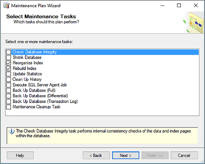
Figure 3-59 Selecting the maintenance tasks to include in the maintenance plan
The Maintenance Task Order page provides the option to change the order in which the tasks are executed. For these two tasks, this should not be ignored and the order in which these two tasks is executed is important.
Recall from the information above that the decision on whether to rebuild or reorganize is based on the percentage of the fragmentation, and the basic rule of thumb is that if the value in this column is between five and 30, you can reorganize the index. Anything over a value of 30 necessitates a rebuild. Thus, you will want to rebuild first as any index with a fragmentation with a percentage of over 30 percent will be caught and addressed first. Then, those indexes over five percent fragmentation are then addressed by the reorganize task, ignoring the other indexes that have just been rebuilt by the rebuild task, because their index fragmentation is now below the threshold.
Make sure the Rebuild Index task is listed first, as shown in Figure 3-60, and then click Next.

Figure 3-60 Setting the order of the maintenance tasks
The next two pages in the wizard are the configuration pages for the rebuild task and the reorganize task. Figure 3-61 shows the Rebuilt Index Task configuration page. On this page, select the databases you want this task to check, whether you want it to check tables, views, or both, and the specific table views to check.
The Default Free Space Per Page option drops the indexes on the tables in the database and re-creates them with the fill factor that was specified when the index was created. The Change Free Space Per Page option drops the indexes on the table and recreates them with a new, automatically calculated fill factor that reserves the specified amount of free space on the index pages. The higher the percentage, the more free space is reserved.
The Keep Index Online option allows users to access the underlying table or indexed data during the index operations, and the Sort Results In Tempdb option determines where the intermediate sort results are stored, which are generated during the index creation.
As discussed, leave the fragmentation and page count values where they are, and click Next.

Figure 3-61 Configuring the rebuild index task
For the Reorganize task, shown in Figure 3-62, configure the databases and objects similar to the Rebuild task, and then configure the other options as needed. The Scan type defines how the system consumes resources while it gathers index statistics. You can choose between consuming less resources (Fast), or more resources (Detailed), depending on how much precision is needed for index statistics. The Optimize Index options are similar to the Rebuild tasks, but be sure to change the Fragmentation percentage to a value around 10, but no less than five, and then click Next.

Figure 3-62 Configuring the reorganize index task
The Select Report Options page simply specifies the options for saving or distributing a report that details the results of the maintenance plan actions. The two options allow the report to be saved to a local file or to be emailed.
The Complete The Wizard page summarizes the configuration. Click Finish, which creates the maintenance plan, and add the tasks to the plan, and add any scheduling options. Because no recurring schedule was defined, you can right-click the maintenance plan and click Execute to run the plan. Creating a recurring schedule for the maintenance plans is discussed later in this skill.
There is one more point to mention before moving on. The values for the fragmentation percent and the page count thresholds are a starting point and these numbers should vary depending on your environment.
Database Engine Tuning Advisor
The Database Engine Tuning Advisor provides insight into the performance of your database by analyzing a workload and the physical implementation of one or more databases. Through a workload analysis, the tuning advisor selects and suggests optimal indexes, indexed views, and partitions without needing to understand the structure of the database.
The workload that the tuning advisor uses is a set of T-SQL statements that the tuning advisor executes against the specified databases you want to analyze and tune. Given the analytical capabilities of the Database Engine Tuning Advisor, it fills some of the gaps that the Maintenance Plan cannot do, such as find missing indexes and recommending indexes that should be removed.
The Database Engine Tuning Advisor can be started from either SQL Server Profiler or from SQL Server Management Studio. In either tool, it is available from the Tools menu by selecting the Database Engine Tuning Advisor menu option.
When the tuning advisor starts, it shows two tabs; the General and Tuning Options tabs. On the General tab, provide a session name, and then select the File option for the workload and browse to the location of a .sql for workload testing. Select the database for workload analysis, then select the database and tables you want to tune, as shown in Figure 3-63.

Figure 3-63 Configuring the General tab of the Database Engine Tuning Advisor
The .sql file selected for the workload analysis should contain one or more SELECT statements, which would represent a decent database workload.
The Tuning Options tab is used to configure the general tuning options. Typically, you won’t need to change much on this page, depending on your SQL environment. For example, do you want the tuning advisor to check both indexes and indexed views, just indexes, or non-clustered indexes? Also, what partitioning strategy do you want to employ during analysis? Most times you won’t need to make any changes, and in this example we just want to analyze the indexes, which is the default configuration setting, shown in Figure 3-64.
The Partitioning Strategy and Physical Design Structures section tell the Tuning Advisor to also look at, ecommend, and change characteristics of the database when looking at tuning options.
The Partitioning Strategy options tell the tuning advisor if and how to look at partitions when performing the analysis. If no partitioning is selected, it will not look at or recommend the use of partitions, whereas Full partitioning will provide recommendations for the use of partitions. The Aligned partitions will recommend partitions that are aligned with existing partitions of underlying tables or view.
The Physical Design Structures section tells the Tuning Advisor whether or not to keep or drop specific structures during analysis.

3-64 Configuring the Tuning Options tab of the Database Engine Tuning Advisor
Once the tuning session has been configured, click the Start Analysis button on the toolbar and the tuning advisor runs the script provided on the General tab to generate a workload and run an analysis of the indexes. By default, the Limit tuning time is checked and the amount of time the analysis runs is one hour. As the analysis is running, a Progress tab appears showing the progress of the analysis.
Once the analysis is complete, two additional tabs appear: Recommendations and Reports, as shown in Figure 3-65.

Figure 3-65 Reviewing the recommendations results
As you can see in Figure 3-65, the tuning analysis revealed that a missing index was identified on the Sales.Invoices table with a recommendation to create the missing index. Likewise, had an index been identified as unused or causing poor performance, that index would have been listed with a value of Drop in the Recommendation column of the results.
The Recommendations tab contains two grids, one for Partition recommendations and another for Index recommendations. The grids do not expand if there are no recommendations.
Given the deep analysis of the Database Engine Tuning Advisor, it solves several of the index maintenance problems identified above including identifying and creating missing indexes, and identifying and removing unused indexes. Updating statistics is addressed later in this skill.
Automate maintenance tasks
Performing regular database maintenance can be a time-consuming process. The skills discussed so far require vigilant watch to ensure that the database runs smoothly and proper database performance is maintained. The skills discussed have focused on indexes and monitoring DMVs, but there are many other tasks that can and should be automated to ensure a well-operating database with proper performance, reliability, and availability.
Database administrators look at automating tasks that they typically repeat on a frequent basis, including:
Database backups
Maintaining indexes
Checking database integrity
Managing database and disk space
Updating statistics
There are several ways to automate many of these tasks, and the following sections discuss two of the more popular approaches: SQL Server Maintenance Plans and PowerShell.
Maintenance plans
SQL Server Maintenance Plans create a workflow of tasks aimed at keeping your database well maintained and optimized. Many of the tasks are grouped together based on functionality to improve task maintenance.
Maintenance plans can be created either by using the user interface in SQL Server Management Studio or via T-SQL. The user interface in SQL Server Management Studio provides the ability to create maintenance plans two ways:
Maintenance Plan Wizard
Maintenance Plan Design Surface
The Maintenance Plan Wizard provides a step-by-step, guided walk-through to create a plan that the SQL Server Agent can run manually or on scheduled basis. You have seen an example of this in this skill when creating a plan to rebuild and reorganize indexes.
The Maintenance Plan Design Surface also creates a maintenance plan but provides the ability to utilize an enhanced workflow and control the workflow steps.
To create a maintenance plan using the design surface, right-click the Maintenance Plans node in the Object Explorer Window in SQL Server Management Studio, and select New Maintenance Plan from the Context menu. In the New Maintenance Plan dialog, provide a name for the maintenance plan, and click OK.
A maintenance plan tab opens in the details section of SQL Server Management Studio, displaying the name and a subplan. A subplan is used where the tasks of the plan are defined, with each subplan able to hold a collection of tasks.
The design surface is similar to SQL Server Integration Services, where tasks are dragged onto the design surface from a toolbox. From the View menu in SQL Server Management Studio, select Toolbox to display the toolbox window that contains all of the maintenance plan tasks. From the Toolbox window, drag the Check Database Integrity Task and Back Up Database Task onto the design surface, as shown in Figure 3-66.

Figure 3-66 Configuring a maintenance plan in the design surface
Each task can be configured by double-clicking the specific task, and configuring the Task Configuration dialog. For example, double-clicking the Database Integrity Task displays the Check Database Integrity Task dialog through which the specific database you want to check is selected and integrity check options are selected. Configure both tasks by double-clicking each task and configuring as appropriate.
As mentioned, the Maintenance Plan Design Surface provides an enhanced workflow and more control over the steps in the workflow, which is not capable to do in the Maintenance Plan Wizard. Thus, additional workflow and decision tree options can be applied, as shown in Figure 3-67. In this example, if the Check Database Integrity Task fails, we don’t want to back up the database, we only want it backed up if the integrity check succeeds. Rather, we would prefer another action be taken if the integrity check fails. As such, as shown in Figure 3-67, we can add another task to the design surface, such as the Notify Operator Task or Execute T-SQL Statement Task, and route to that task given the failure of the database integrity check.

Figure 3-67 Configuring detailed task workflow
To schedule the maintenance plan, click the Job Schedule Properties button on the subplan and configure the frequency in which the plan will run in the Job Schedule Properties dialog. Click OK on the dialog, and then save the maintenance plan.
Once the maintenance plan is saved it appears underneath the Maintenance Plans node. Additionally, each subplan created appears in the Jobs node underneath the SQL Server Agent node, as shown in Figure 3-68.

Figure 3-68 The maintenance plan and correlated job in object explorer
Keep in mind that each maintenance plan can have multiple subplans, and each subplan shows up as a job within the Jobs node.
PowerShell
Windows PowerShell is a Windows command-line, interactive prompt and scripting environment built on top of the .NET Framework and has quickly become a great tool for automating tasks of all kinds, including operating system as well as SQL Server.
PowerShell is very powerful and there are many ways to use PowerShell to automate SQL tasks. As versatile as it is, it can be very verbose, meaning that it sometimes can take a lot of code to accomplish some tasks. As such, only code-snippets are supplied and links to full source code samples are provided.
You can find a sample PowerShell script that uses the Standard .NET Framework classes to connect to a specific database instance to rebuild and reorganize indexes at https://gallery.technet.microsoft.com/scriptcenter/SQL-Optimization-In-95d12ce6.
Many of the examples you find online use the SQL Server Management Objects (SMO) because it makes it easy to navigate and iterate through the databases of a SQL Server instance and their objects, and then use the SMO index object like this:
$index.Rebuild()
$index.Reorganize()
The following code snipped provides a high-level sample of iterating the objects, checking their fragmentation level, and either rebuilding or re-indexing based on the results.
$v = [System.Reflection.Assembly]::LoadWithPartialName( 'Microsoft.SqlServer.SMO')
$smo = new-object ('Microsoft.SqlServer.Management.Smo.Server') $inst
$dbs = $smo.Databases

foreach ($db in $dbs) {
$tbs = $db.Tables
foreach ($tb in $tbs) {
$ixs = $tb.Indexes
foreach ($ix in $ixs) {

# Get the Fragmentation and page count information
$q = @"
SELECT avg_fragmentation_in_percent, page_count FROM sys.dm_db_index_physical_stats($dbid, $tbid, $ixid, NULL, NULL)
"@

$res = invoke-sqlcmd -ServerInstance $inst -Database $dbname -Query $q
$frval = $res.avg_fragmentation_in_percent
$pgcnt = $res.page_count

if ($frval -gt 30 -and $pgcnt -gt 1000) {
$ix.Rebuild()
}
elseif ($frval -gt 10 -and $pgcnt -gt 1000) {
$ix.Reorganize()
}
}
}
}
Obviously this code snippet is not complete, but it provides insight on how you can use PowerShell to accomplish many of the maintenance tasks discussed. Once the PowerShell script is tested appropriately, it can be scheduled several ways, such as using the Windows scheduler, or through a SQL Server job.
Update statistics
The query optimizer uses statistics to create query plans to improve query performance. Most of the time, the query optimizer has already generated the necessary statistics for an optimal query plan, but there are times where additional statistics are necessary or the existing statistics need updating for a better query plan.
For the query optimizer, statistics contain information about the distribution of values in one or more columns of a table or indexed view. The query optimizer uses these statistics to estimate the cardinality, or number of rows, in the query result. The cardinality estimates are generated by the cardinality estimator and are used to create a high-quality query plan. If the cardinality estimates are off, resulting in poor statistics, the result could be the difference between a poor performing and resource-intensive index scan versus the better performing index seek.
Statistics can be updated several ways. In many environments, statistics are updated via a maintenance plan that provides a proactive approach to updating statistics. When creating a maintenance plan using the Maintenance Plan Wizard, select the Update Statistics option on the Select Maintenance Tasks page. The Define Update Statistics Task page then allows you to configure the maintenance task, shown in Figure 3-69.

Figure 3-69 Configuring the update statistics task
Index statistics are created automatically when the index is created. Column statistics are created manually using the CREATE STATISTICS statement, or they are created automatically if the Auto Create Statistics option is set to True.
The Scan type defines the amount of data used to determine the statistic. The Full scan option costs more resource time, but ensures that the statistics are accurate. The Sample By option uses the percentage of the rows specified and extrapolates the rest, resulting in a faster update of the statistics but the statistics may not be accurate. As such, the Full scan is recommended, but updating statistics should be done off hours.
The query optimizer is quite smart. It determines when the statistics might be out of date and updates them as needed for a query plan. This option is on by default via a database-level setting, the Auto Update Statistics configuration setting, shown in Figure 3-70.

Figure 3-70 The auto update statics option in the Database Properties dialog
The question then becomes when to update statistics. If the query optimizer is so smart, why do statistics need to be updated via a DBA? As smart as the query optimizer is, it is not perfect. It does its best, but there are times when query plans can be improved, thus improving query performance, by updating statistics more frequently than the Auto Update Statistics setting dictates. Statistics become out of date after INSERT, UPDATE, DELETE, and MERGE operations change the data distribution in the table or indexed view, and the query optimizer determines their out of date by counting the number of data modifications since the latest statistics update, and comparing the number of modifications to the number of rows in the table or indexed view.
A great way to determine when statistics were last updated is by looking at the last_updated column in the sys.dm_db_stats_properties DMV, as shown in Figure 3-71.

Figure 3-71 Checking when statistics were last updated
The STATS_DATE function is also useful as it returns similar information, but broken out by index.
Updating statistics causes queries to recompile, so it is recommended to not update statistics too frequently due to the performance tradeoff between improving query plans and query recompile time.
Therefore, consider the following when deciding when to update statistics:
Slow query performance If queries have a slow or unpredictable response time over a period of time, look at the statistics.
After maintenance operations Some maintenance operations change the distribution of data, such as table truncations or bulk inserts.
Insert operations on ascending or descending columns Appending new rows to ascending or descending columns, such as IDENTITY columns, might be too small to trigger an automatic statistics update.
Updating statistics can also be updated using T-SQL. The following T-SQL statement updates the statistics for all the indexes on the Sales.Invoices table in the WideWorldImporters database.
UPDATE STATISTICS Sales.Invoices;
The following T-SQL statement updates the statistics for all the FK_Sales_Invoices_OrderID index on the Sales.Invoices table in the WideWorldImporters database.
UPDATE STATISTICS Sales.Invoices AK_Sales_Invoices_OrderID;
Updating statistics should not be overlooked. It should be a regular part of your maintenance plan strategy, simply because issues like bad parameter sniffing can be alleviated with better statistics
Verify database integrity
A few years ago a member of the Microsoft SQL Server product support team published a blog post and it stated that more than 95 percent of all corruption cases turned out to be caused by a platform issue, the layer below SQL Server. The primary cause was a firmware bug, or third-party driver, with the second most common cause being actual hardware failure. The idea is that many things can cause database corruption, such as damage to the hard drive, environmental factors and influences, normal hardware wear and tear, or bad data in general.
The question isn’t if database corruption will happen, it’s when. Database corruption will happen at some point. The focus is on the things you should be doing to proactively monitor for database corruption and how to address it when it does happen.
The following two sections discuss the options available to proactively monitor for database corruption and to check and verify database integrity.
Maintenance plan
This skill has covered SQL Server Maintenance plans quite a bit, and for good reason. They provide a proactive and quick way to get insight into the status of your database. Checking the integrity of your database is no different because a maintenance plan task exists that checks the integrity of your database.
The Check Database Integrity Task checks the allocation and structural integrity of all the objects in a specified database, or multiple database. Additionally, the task can check the integrity of all the index and table data pages.
When creating a maintenance plan using the Maintenance Plan Wizard, select the Check Database Integrity option on the Select Maintenance Tasks page. The Define Database Check Integrity Task page then allows you to configure the maintenance task, shown before in Figure 3-72.

Figure 3-72 Configuring the Database Check Integrity task
Behind the scenes, the Check Database Integrity Task encapsulates the DBCC CHECKDB statement, providing a user-interface to configure, schedule, and run the DBCC CHECKDB statement.
The benefit of using a maintenance plan is that, as you learned earlier, you can include this plan as part of an overall workflow and take action based on the outcome of the task.
DBCC CHECKDB
The DBCC CHECKDB statement accomplishes the same functionality as the maintenance plan, with the difference being that you are running a T-SQL statement with the output being returned in the output window. The DBCC CHECKDB statement checks the logical and physical integrity of all the objects. It does this by also executing additional DBCC statements:
DBCC CHECKALLOC Checks the consistency of disk space allocation.
DBCC CHECKTABLE Checks the integrity of all the pages and structures that make up the table or indexed view.
DBCC CHECKCATALOG Checks the catalog consistency.
DBCC CHECKDB also validates the contents of every indexed view in the database and validates link-level consistency between table metadata and file system directories.
To run DBCC CHECKDB, execute the statement in a query window, as shown in Figure 3-73. As you can see, CHECKDB found 0 allocation errors and 0 consistency checks in the database. Also notice that the scrollbar in the results window is scrolled quite a ways down to the end of the output, so the amount of output is significant.

Figure 3-73 Running DBCC CHECKDB in a query window
The example above runs DBCC CHECKDB for the current database, but you can also specify the database to check:
DBCC CHECKDB ([WideWorldImporters])
There are certain benefits to checking database integrity using the DBCC CHECKDB statement because there are several parameters you can pass to the statement, such as the REPAIR_REBUILD parameter, which performs repairs that have no possibility of data loss, including repairing missing rows in non-clustered indexes, and rebuilding indexes.
One of the parameters that is available to use with DBCC CHECKDB is called REPAIR_ALLOW_DATA_LOSS. This option tells DBCC CHECKDB to try and repair all reported errors, even if it means data loss. As such, it is recommended that this be used only in a “worst case” scenario. The recommended approach is to restore the database from the last known good backup and not use this parameter.
The idea behind verifying database integrity is to detect database correction as early as possible. If database corruption goes undetected long enough it could, and probably will, lead to data loss. There is nothing you can do to prevent database corruption. As stated earlier, it’s not a matter of if, but when. The goal is to detect it as soon as possible so corrective action can be taken, and DBCC CHECKDB is the best way to detect it, whether you run it via T-SQL or a maintenance plan.
The question you should be asking yourself is: How often should you validate database integrity and run consistency checks? To answer that question, you need to look at your environment. Is your I/O subsystem pretty flaky or is it the most reliable thing on the planet? Do you have solid backup strategy or no backup strategy at all? If you do take regular backups, how confident are you that you can recover from corruption with little to no downtime?
The answers to these questions depends on how often you should verify database integrity. You might be comfortable running consistency checks weekly if you have faith in your environment and are a rock star with your backups and backup strategy. If you are on the opposite end of the spectrum, you might want to consider changing your ways.
The good thing is that, regardless of whether or not you use T-SQL or the maintenance plan, you can schedule the consistency check easily to run on a regular schedule, and you should do so.
Recover from database corruption
Database corruption is inevitable. As mentioned previously, it is not a matter of if, but when. You have done your best to monitor and prevent database corruption, but it happened. They say that the best offense is a good defense, and this absolutely applies here. Recovering from database corruption is all about applying a defensive strategy to make recovery a winning situation.
Before discussing recovery, let’s take a moment to talk about a good backup plan and strategy. The last thing you want is to find out in the middle of a production recovery situation that you have no backups or your backups are worthless.
As a rule of thumb, database backups should follow these best practices:
Full backups In most cases, a full database backup should be performed weekly. These can be performed online.
Differential backups Captures only the data that has changed since the most recent, full backup.
Transaction log backups Transaction logs contain all the recent activity and can be used to restore a database back to a specific point in time. They also can be performed online. Backup frequency depends on activity.
System databases Weekly for stable installations.
A backup strategy is incomplete without backing up the system databases. The system databases contain a lot of information, such as system configuration and SQL Server job information. Depending on how frequent your database changes are, you might consider a daily or weekly backup frequency.
Transaction log backups depend on how active your database is. A database with heavy transactions might look at backing up the transaction log every 10, 15, or 30 minutes. Less active database might look at backing up the transaction log every one or two hours.
Additionally, when backing up, consider using advanced features such as checksum to detect problems with the backup media itself. Checksum specifies that the backup operation verifies each page for checksum and torn page and generates a checksum for the entire backup.
Part of having a good backup strategy also consists of knowing where to back them up to. Make sure you are not storing your backups in the same physical location as the database files. If the physical drive goes bad, you can use other drives or remote locations that stored the backups to perform a restore.
Now that you have your backup strategy in place, the next step is to practice recovery operations. Just because backups were taken and the backup process succeeded doesn’t mean that all is well. Without practicing and walking through the recovery process in its entirety you cannot be entirely sure of the integrity of the backups.
Therefore, have a test server on hand, or in the cloud, to frequently test your backups and your restore strategy, and follow a restore process that you would follow in a production, real-life situation. This minimizes any problems that occur during an actual corruption issue.
With all of that as a foundation, our attention should now focus on the steps necessary to recovery from a corrupted database.
The first step is to run CHECKDB and review the output results because you need to know where the corruption is. If you used a maintenance plan to run CHECKDB, write the output to a file so you have a copy. Review it thoroughly to understand what the issues are and where the corruption is. CHECKDB provides the necessary information to what the problem is, and in what object the corruption exists.
Depending where the corruption is will depend on what the steps are to recover. If the corruption exists in a non-clustered index for example, rebuilding the index just might solve the problem and you’re on your way. To fix the index, you need to disable the index by running the ALTER INDEX statement. For example:
ALTER INDEX IX_Sales_OrderID ON Sales.Invoices DISABLE;
Next, rebuild the index by again using the ALTER INDEX statement, this time specifying to rebuild online.:
ALTER INDEX IX_Sales_OrderID ON Sales.Invoices REBUILD WITH ONLINE=ON;
This will go through the process of recreating the index and fix any corruption issues. Rerun the CHECKDB again to see if the corruption has been fixed.
If the corruption exists in a data table or other object, you will most likely be looking at restoring the database. You could potentially be looking at repairing the database, but at the cost of losing data, so a repair option should not be considered at this point in the recovery process.
To recover through a database restore, the first step is to make a tail-log backup. A tail-log backup captures any transaction log records that were written to the transaction log since the last time it was backed up.
To back up the tail of the transaction log, right-click the corrupted database and from the context menu select Tasks -> Back Up. In the Back Up Database dialog, set the Backup type to Transaction Log, then on the Media Options page in the Reliability section make sure the Verify Backup When Finished And Perform Checksum Before Writing Media options are checked. Then in the Transaction log section, check the Back Up The Tail Of The Log, as shown in Figure 3-74.

Figure 3-74 Configuration options for restoring the tail of the transaction log
If you have followed a best-practices backup strategy and have full and transaction log backups, the next step is to review your backups to identify when the corruption occurred. Again, this is where a best-practices restore strategy, and a test server, comes into play.
Take the most recent full backup and restore it on the test server, running CheckDB on it, and then repeating the process with the next previous full backup until you find the backup that was made before the corruption occurred. At this point, depending on the error returned by CHECKDB and the object on which the corruption exists, the option might exist to restore a page or filegroup which will be faster and in a lot of cases be performed while the database is still online.
Page and File/Filegroup objects can be restored by right-clicking the corrupted database and select Restore > Page or File And FileGroups, as shown in Figure 3-75.

Figure 3-75 The menu option to restore a specific data page
The goal of the page restore is to restore one or more damaged pages without restoring the whole database. Pages that are candidates for restore have been marked as “suspect” and the Restore Page dialog helps restore those from backupsets. SQL Server maintains an internal table called the Suspect_Pages table, which is used for maintaining information about suspect pages, and provides information that helps decide whether a restore is necessary. This table resides in the msdb database.
If the corruption is beyond the ability to restore a page or filegroup, a full database restore is needed. Again, on a test server, review your backups to identify when the corruption occurred and find the backup that was made before the corruption occurred. Then, restore all of the transaction log backups, then finally the tail-log backup.
Run CHECKDB again to ensure the corruption does not exist and the problem has been properly and efficiently solved. Again, the CHECKDB repair option should be used as a last option if the restore process was not successful. However, when following database back up best practices and an appropriate backup and restore strategy have been implemented and practiced, restoring the database as discussed has high success rates.
Once you are confident in the process and the resolution, perform the same restore options on the production server, preferably not during production hours.
With the database back online and operating normally, it would be beneficial to take some time to explore potential reasons of what initially caused the corruption. Could the corruption have been avoided, and if so, how? Take this time to do a thorough inspection of both hardware and software to uncover the reason for the corruption. For example, you can look at the page with a hex editor and possibly fix the problem, or hack-attach the suspect database, which is re-attaching a damaged database if it has been accidentally detached.
The point to take away here is that database corruption happens but it can be reduced greatly by having a solid back up strategy along with regular overall health monitoring.
Thought experiment
In this thought experiment, apply what you’ve learned about in this Chapter. You will find the answers to these questions in the next section.
You are a consultant to the Contoso Corporation. Contoso is an enterprise-level company that has a customer facing ordering system. The number of orders continues to grow and the size of the database is growing exponentially. The size of the database is reaching 400 GB, and much of that is old historical data, but the amount of new data grows rapidly on a daily basis and users have reported slower response times in the application.
Company policy states that records should be kept for a period of time, but Contoso’s CIO states that storage cost is becoming an issue. In addition, the CIO has asked the DBAs to look at the performance issue and they have applied several indexes without any change in performance. The CIO has also reported that their current hardware is getting old and several hardware issues on the SQL Server box has appeared and he is unsure if they have a proper recovery plan in place.
What can Contoso due to address the storage cost issue while still keeping their cold data?
How should Contoso address their application performance problems?
What should Contoso’s recovery approach be?
How should Contoso approach be in defining a maintenance strategy?
Thought experiment answers
This section provides the solution to the thought experiment. Each answer explains why the answer is correct.
Contoso should use Stretch Database to migrate all their historical data to Azure. This will require no application changes, free up disk space locally, and still meet security and company policy.
In addition to reviewing existing code, Contoso should use many of the dynamic management views as well as the Database Engine Tuning Advisor to help identify missing indexes and remove unused indexes. Contoso should also look at query statistics. Contoso should also look at and validate existing hardware infrastructure.
Contoso should ensure that an appropriate backup and recovery strategy is in place for their environment. Contoso should regularly test this strategy in a test environment to ensure a successful strategy.
Contoso should define and implement a maintenance schedule which includes verifying database integrity and performing index maintenance and updating statistics.
Chapter summary
The SMB 3.0 protocol included optimizations that SQL Server can take advantage of, including significant performance enhancements and improvements.
The SMB 3.0 protocol comes with Windows Server 2012 and later versions.
The Stretch Database feature was added to SQL Server 2016 to provide cost efficient storage of cold data.
Stretch Database can be implemented without any changes to the application.
The remote table for Stretch Database can be optimized with a performance tier like any other Azure SQL database.
An Azure storage account comes with blob, table, queue, and file storage services.
The Azure file share service, part of an Azure storage account, provide the ability to create fully managed file shares that are accessible via the SMB protocol.
Azure file shares can be mounted both on-premises and in the cloud.
Azure SQL Database service tiers provide flexibility in changing performance and storage levels based on database workload.
Azure SQL Database service tiers can be changed to meet the workload demands with little to no downtime.
SQL Server includes many dynamic management views through which to track and review wait statistics.
SQL Server tracks wait for information to help troubleshoot and track down performance issues.
Storage pools, introduced in Windows Server 2012, allow the grouping of physical disks into a resource pool.
Virtual disks, called storage spaces, can be created from the resources within a storage pool.
Index maintenance is a critical part of database maintenance to ensure a well-performing database.
Index maintenance includes removing index fragmentation, identifying missing indexes, and removing unused indexes.
Maintenance tasks can be used to monitor and maintain many aspects of SQL Server, including indexes, statistics, and database integrity.
Database integrity should be performed often on a regular schedule.
A proper backup and restore strategy should be created, maintained, and tested to be able to recover from database corruption.