
7
Application of Sub‐Population Scheduling Algorithm in Multi‐Population Evolutionary Dynamic Optimization
Javidan Kazemi Kordestani1 and Mohammad Reza Meybodi2
1 Department of Computer Engineering, Science and Research Branch, Islamic Azad University, Tehran, Iran
2 Soft Computing Laboratory, Computer Engineering and Information Technology Department, Amirkabir University of Technology (Tehran Polytechnic), Tehran, Iran
7.1 Introduction
Many problems in real‐world applications involve optimizing a set of parameters, in which the objectives of the optimization, some constraints, or other elements of the problems may vary over time. If so, the optimal solution(s) to the problems may change as well. Generally speaking, various forms of dynamic behavior are observed in a substantial part of real‐world optimization problems in different domains. Examples of such problems include the dynamic resource allocation in shared hosting platforms [1], dynamic traveling salesman problem that changes traffic over time [2], dynamic shortest path routing in MANETs [3], aerospace design [4], pollution control [5], ship navigation at sea [5], dynamic vehicle routing in transportation logistics [6], autonomous robot path planning [7], optimal power flow problem [8], dynamic load balancing [9], and groundwater contaminant source identification [10].
Evolutionary computation (EC) techniques have attracted a great deal of attention due to their potential for solving complex optimization problems. Even though they are effective for static optimization problems, they should undergo certain adjustments to work well when applied to dynamic optimization problems (DOPs). The reason is that the dynamic behavior of DOPs poses two additional challenges to the EC techniques: (i) outdated memory: when a change occurs in the environment, the previously found solutions by the algorithm may no longer be valid. In this case, the EC algorithm will be misled into moving toward false positions. (ii) Diversity loss: this issue appears due to the tendency of the population to converge to a single optimum. As the result, when the global optimum is shifted away, the number of function evaluations (FEs) required for a partially converged population to relocate the optimum is quite deleterious to the performance.
While both the above challenges can be detrimental to the performance of EC, the second issue is far more serious.
Over the years, researchers have proposed various techniques to improve the efficiency of traditional EC methods for solving DOPs. According to [11] the existing proposals can be categorized into the following six approaches:
- increasing the diversity after detecting a change in the environment [12–14];
- maintaining diversity during the optimization process [15, 16];
- employing memory schemes to retrieve information about previously found solutions [17, 18];
- predicting the location of the next optimal solution(s) after a change is detected [19, 20];
- making use of the self‐adaptive mechanisms of ECs [21, 22];
- using multiple sub‐populations to handle separate areas of the search space concurrently [23–35].
Among the above mentioned approaches, the multi‐population approach has been shown to be very effective for handling DOPs, especially for multi‐modal fitness landscapes. The success of this approach can be attributed to three reasons [36]:
- As long as different populations search in different sub‐areas in the fitness landscape, the overall population diversity can be maintained at the global level.
- It is possible to locate and track multiple changing optima simultaneously. This feature can facilitate tracking of the global optimum, given that one of the being‐tracked local optima may become the new global optimum when changes occur in the environment.
- It is easy to extend any single‐population approach, e.g. diversity increasing/maintain schemes, memory schemes, adaptive schemes, etc. to the multi‐population version.
Although effective, the multi‐population approach significantly reduces the utilization of FEs and delays the process of finding the global optimum by sharing an equal portion of FEs among sub‐populations. In another words, sub‐populations located far away from the optimal solution(s) are assigned the same amount of FEs as those located near to optimal solution(s), which in turn exert deleterious effects on the performance of the optimization process.
Since the calculation of FEs is the most expensive component of the EC methods for solving real‐world DOPs, dynamic optimization can be considered as scheduling the sub‐populations in a way that the major portion of FEs is consumed around the most promising areas of the search space. Therefore, one major challenge is how to suitably assign the FEs to each sub‐population to enhance the efficiency of multi‐population methods for DOPs.
This chapter is aimed at providing the application of scheduling in enhancing the performance of multi‐population methods for tracking optima in DOPs. Eight different sub‐population scheduling (SPS) algorithms, which have been applied to a well‐known multi‐population algorithm called DynDE, will be evaluated and compared using one of the most widely used benchmarks in the literature.
7.2 Literature Review
As mentioned earlier in this chapter, the multi‐population is one of the most efficient approaches to tackle the existing challenges in DOPs. The idea behind this is to divide the individuals (candidate solutions) of the main population into multiple sub‐populations so they can search in different sub‐areas of the fitness landscape in parallel. In this way, the algorithm is able to efficiently handle several issues arising in DOPs: (i) exploration, (ii) optimum tracking, (iii) change detection, and (iv) premature convergence. In the rest of this section, we provide a literature review on multi‐population methods for DOPs.
7.2.1 Multi‐Population Methods with a Fixed Number of Populations
The main idea of these methods is to divide the task of optimization among a number of fixed‐size populations. One way to do this is by establishing a mutual repulsion among a predefined number of sub‐populations to place them over different promising areas of the search space. The representative work in this category is that of Blackwell and Branke [37]. They proposed two multi‐swarm algorithms based on the particle swarm optimization (PSO), namely mCPSO and mQSO. In mCPSO, each swarm is composed of neutral and charged particles. Neutral particles update their velocity and position according to the principles of pure PSO. On the other hand, charged particles move in the same way as neutral particles, but they are also mutually repelled from other charged particles residing in their own swarm. Therefore, charged particles help to maintain the diversity inside the swarm. In mQSO, instead of having charged particles, each swarm contains quantum particles. Quantum particles change their positions around the center of the best particle of the swarm according to a random uniform distribution with radius rcloud . Consequently, they never converge and provide a suitable level of diversity to swarm in order to follow the shifting optimum. The authors also introduced the exclusion operator, which prevents populations from settling on the same peak. In another work [23], the same authors proposed a second operator referred to as anti‐convergence, which is triggered after all swarms converge and reinitializes the worst swarm in the search space. After the introduction of mQSO, a lot of work has been done to enhance its performance by modifying various aspects of its behavior.
A group of studies analyzed the effect of changing the number and the distribution of quantum particles on the performance of mQSO. For instance, Trojanowski [38] proposed a new class of limited area distribution for quantum particles in which the uniformly distributed candidate solutions within a hyper‐sphere with radius rcloud are wrapped using von Neumann's acceptance‐rejection method. In another work [39], the same author introduced a two‐phased method for generating the cloud of quantum particles in the entire area of the search space based on a direction vector θ and the distance d from the original position using an α‐stable random distribution. This approach allows particles to be distributed equally in all directions. The findings of both studies revealed that changing the distribution of quantum particles has a significant effect on the performance of mQSO. del Amo et al. [40] investigated the effect of changing the number of quantum and neutral particles on the performance of mQSO. The three major conclusions of their study can be summarized as follows: (i) an equal number of quantum and neutral particles is not the best configuration for mQSO, (ii) configurations in which the number of neutral particles is higher than the number of quantum particles usually perform better, and (iii) quantum particles are most helpful immediately after a change in the environment.
Some researchers borrowed the general idea of mQSO and developed it using other ECs. The main purpose of these approaches is to benefit from intrinsic positive characteristics of other algorithms to reach a better performance than the mQSO. For instance, Mendes and Mohais [41] introduced a multi‐population differential evolution (DE) algorithm, called DynDE. In DynDE several populations are initialized in the search space and explore multiple peaks in the environment incorporating exclusion. DynDE also includes a method for increasing diversity, which enables the partially converged population to track the shifting optimum.
One of the technical drawbacks of the exclusion operator in mQSO is that it ignores the situations when two populations stand on two distinct but extremely close optima (i.e. within the exclusion radius of each other). In these situations, the exclusion operator simply removes the worst population and leaves one of the peaks unpopulated. A group of studies tried to address this issue by adding an extra routine to the exclusion which is executed whenever a collision is detected between two populations. For example, Du Plessis and Engelbrecht [42] proposed re‐initialization midpoint check (RMC) to detect whether different peaks are located within the exclusion radius of each other. In RMC, once a collision occurs between two populations, the fitness of the midpoint on the line between the best individuals in each population is evaluated. If the fitness of the midpoint has a lower value than the fitness value of the best individuals of both populations, it implies that the two populations reside on distinct peaks and that neither should be reinitialized. Otherwise, the worst‐performing population will be reinitialized in the search space. Although RMC is effective, as pointed by the authors, it is unable to correctly detect all extremely close peaks. In another work, Xiao and Zuo [43] applied hill‐valley detection with three checkpoints to determine whether two colliding populations are located on different peaks. In their approach, three points between the best solutions of the collided populations x and y are examined. Thereafter, if there exists a point z = c · x + (1 − c) · y for which f(z) < min {f(x), f(y)}, where cϵ{0.05, 0.5, 0.95}, then two populations are on different peaks and they remain unchanged. Otherwise, they are on the same peak.
Another interesting approach for improving the performance of mQSO is to spend more FEs around the most promising areas of the search space. In this regard, Novoa‐Hernández et al. [44] proposed a resource management mechanism, called swarm control mechanism, to enhance the performance of the mQSO. The swarm control mechanism is activated on the swarms with low diversity and bad fitness, and stops them from consuming FEs. In another work, Du Plessis and Engelbrecht [45] proposed an extension to the DynDE referred to as favored populations DE. In their approach, FEs between two successive changes in the environment are divided into three phases: (i) all populations are evolved according to normal DynDE for ζ1 generations in order to locate peaks, (ii) the weaker populations are frozen and stronger populations are executed for another ζ2 generations, and (iii) frozen populations are put back to the search process and all populations are evolved for ζ3 generations in a normal DynDE manner. This strategy adds three parameters ζ1, ζ2, and ζ3 to DynDE, which must be tuned manually.
The SPS, which is the subject of this chapter, falls under this category where the main objective is to distribute FEs among the sub‐populations so as to allocate the greatest amount of FEs to the most successful sub‐populations. Despite the progress achieved in the past, we believe that there is still room for improving this approach. Therefore, this chapter focuses on different ways to suitably assign FEs to each sub‐population using the SPS algorithm.
Different from the above studies, some researchers combined desirable features of various optimization algorithms into a single collaborative method for DOPs. In these methods, each population plays a different role and information can be shared between populations. For example, Lung and Dumitrescu [46] introduced a hybrid collaborative method called collaborative evolutionary‐swarm optimization (CESO). CESO has two equal‐size populations: a main population to maintain a set of local and global optimum during the search process using crowding‐based DE, and a PSO population acting as a local search operator around solutions provided by the first population. During the search process, information is transmitted between both populations via collaboration mechanisms. In another work [47] by the same authors, a third population is incorporated to CESO which acts as a memory to recall some promising information from past generations of the algorithm. Inspired by CESO, Kordestani et al. [48] proposed a bi‐population hybrid algorithm. The first population, called QUEST, is evolved by crowding‐based DE principles to locate the promising regions of the search space. The second population, called TARGET, uses PSO to exploit useful information in the vicinity of the best position found by the QUEST. When the search process of the TARGET population around the best‐found position of the QUEST becomes unproductive, the TARGET population is stopped and all genomes of the QUEST population are allowed to perform an extra operation using hill‐climbing local search. They also applied several mechanisms to conquer the existing challenges in the dynamic environments and to spend more FEs around the best‐found position in the search space.
7.2.2 Methods with a Variable Number of Populations
Another group of studies has investigated the multi‐population schemes with a variable number of sub‐populations. These methods can be further categorized into three groups based on how the sub‐populations are formed from a main population. They are methods with a parent population and variable number of child populations, methods based on population clustering, and methods based on space partitioning.
7.2.2.1 Methods with a Parent Population and Variable Number of Child Populations
The first strategy to make a variable number of populations is to split off sub‐populations from the main population. The major strategy in this approach is to divide the search space into different sub‐regions, using a parent population, and carefully exploit each sub‐region with a distinct child population. Such a method was first proposed by Branke et al. [49]. Borrowing the concept of forking, they proposed a multi‐population genetic algorithm for DOPs called self‐organizing scouts (SOS). In SOS, the optimization process begins with a large parent population exploring through the whole fitness landscape with the aim of finding promising areas. When such areas are located by the parent, a child population is split off from the parent population and independently explores the respective sub‐space, while the parent population continues to search in the remaining search space for locating new optimum. The search area of each child population is defined as a sphere with radius r and centered at the best individual. In order to determine the number of individuals in each population, including the parent, a quality measure is calculated for each population as defined in [49]. The captured region by the child population is then isolated by re‐initializing individuals in the parent population that fall into the search range of the child population. In SOS, overlapping among child populations is usually accepted unless the best individual of a child population falls within the search radius of another population. In this case, the whole child population is removed.
Later, similar ideas were proposed by other authors. For instance, Yang and Li [34] proposed a fast multi‐swarm algorithm for DOPs. Their method starts with a large parent swarm exploring the search space with the aim to locate promising regions. If the quality of the best particle in the parent swarm improves, it implies that a promising search area may be found. Therefore, a child swarm is split off from the parent swarm to exploit its own sub‐space. The search territory of each child swarm is determined by a radius r which is relative to the range of the landscape and width of the peaks. If the best particle of one child swarm approaches the area captured by another child swarm, the worse child swarm will be removed to prevent child populations residing on the same peak. Besides, if a child swarm fails to improve its quality in a certain number of iterations, the best particle of the child swarm jumps to a new position according to a scaled Gaussian distribution. Another similar approach can be found in [27]. An interesting approach is the hibernating multi‐swarm optimization algorithm proposed by Kamosi et al. [26], where unproductive child swarms are stopped using a hibernation mechanism. In turn, more FEs will be available for productive child swarms.
Yazdani et al. [50] employed several mechanisms in a multi‐swarm algorithm for finding and tracking the optima over time. In their proposal, a randomly initialized finder swarm explores the search space for locating the position of the peaks. In order to enhance the exploitation of promising solutions, a tracker swarm is activated by transferring the fittest particles from the finder swarm into the newly created tracker swarm. Besides, the finder swarm is then reinitialized into the search space to capture other uncovered peaks. Afterward, the activated tracker swarm is responsible for finding the top of the peak using a local search along with following the respective peak upon detecting a change in the environment. In order to avoid tracker swarms exploiting the same peak, exclusion is applied between every pair of tracker swarms. Besides, if the finder swarm converges to a populated peak, it is reinitialized into the search space without generating any tracker swarm.
Recently, Sharifi et al. [33] proposed a hybrid approach based on PSO and local search. In this method, a swarm of particles is used to estimate the location of the peaks. Once the swarm has converged, a local search agent is created to exploit the respective region. Moreover, a density control mechanism is used to remove redundant local search agents. The authors also studied three adaptations to the basic approach. Their reported results clearly indicate the importance of managing FEs to reach a better performance.
7.2.2.2 Methods Based on Population Clustering
Differing from the above algorithms where the sub‐populations are split off from the main population, another way to create multiple populations is to divide the main population of the algorithm into several clusters, i.e. sub‐populations, via different clustering methods. For instance, Parrott and Li [51] proposed a speciation‐based PSO for tracking multiple optima in dynamic environments, which dynamically distributes particles of the main swarm over a variable number of so‐called species. In [52] the performance of speciation‐based PSO was improved by estimating the location of the peaks using a least squares regression method.
Similarly, Yang and Li [35] proposed a clustering PSO (CPSO) for locating and tracking multiple optimums. CPSO employed a single linkage hierarchical clustering method to create a variable number of sub‐swarms, and assign them to different promising sub‐regions of the search space. Each created sub‐swarm uses the PSO with a modified gbest model to exploit the respective region. In order to avoid different clusters from crowding, they applied a redundancy control mechanism. In this regard, when two sub‐swarms are located on a single peak they are merged together to form a single sub‐swarm. So, the worst performing individuals of the sub‐swarm are removed until its size is equal to a predefined threshold. In another work [53], the fundamental idea of CPSO is extended by introducing a novel framework for covering undetectable dynamic environments.
In [54] a competitive clustering PSO for DOPs is introduced. It employs a multi‐stage clustering procedure to split the particles of the main swarm. Then, the particles are assigned to a varying number of sub‐swarms based on the particles' positions and their objective function values. In addition to the sub‐swarms, there is also a group of free particles that is used to explore the environment to locate new emerging optimums or track the current optimums which are not followed by any sub‐swarm. Recently, Halder et al. [55] proposed a cluster‐based DE with external archive which uses k‐means clustering method to create a variable number of populations.
7.2.2.3 Methods Based on Space Partitioning
Another approach for creating multiple sub‐populations from the main population is to divide the search space into several partitions and keep the number of individuals in each partition less than a predefined threshold. In this group, we find the proposal of Hashemi and Meybodi [25]. Here, cellular automata are incorporated into a PSO algorithm (cellular PSO). In cellular PSO, the search space is partitioned into some equally sized cells using cellular automata. Then particles of the swarm are allocated to different cells according to their positions in the search space. Particles residing in each cell use their personal best positions and the best solution found in their neighborhood cells for searching an optimum. Moreover, whenever the number of particles within each cell exceeds a predefined threshold, randomly selected particles from the saturated cells are transferred to random cells within the search space. In addition, each cell has a memory that is used to keep track of the best position found within the boundary of the cell and its neighbors. In another work [24], the same authors improved the performance of cellular PSO by changing the role of particles to quantum particles just at the moment when a change occurs.
Inspired by the cellular PSO, Noroozi et al. [30] proposed an algorithm based on DE, called CellularDE. CellularDE employs the DE/rand‐to‐best/1/bin scheme to provide local exploration capability for genomes residing in each cell. After detecting a change in the environment, the population performs a random local search for several upcoming iterations. In another work [31], the authors improved the performance of CellularDE by using a peak detection mechanism and hill climbing local search.
7.2.3 Methods with an Adaptive Number of Populations
The last group of studies includes methods that control the search progress of the algorithm and adapt the number of populations based on one or more feedback parameters.
The critical drawback of the multi‐swarm algorithm proposed in [23] is that the number of swarms should be defined before the optimization process. This is a clear limitation in real‐world problems where information about the environment might be not available. The very first attempt to adapt the number of populations in dynamic environments was made by [56]. He developed an adaptive mQSO (AmQSO) which adaptively determines the number of swarms either by spawning new swarms into the search space, or by destroying redundant swarms. In this algorithm, swarms are categorized into two groups: (i) free swarms, whose expansion, i.e. the maximum distance between any two particles in the swarm in all dimensions, is larger than a predefined radius rconv, and (ii) converged swarms. Once the expansion of a free swarm becomes smaller than a radius rconv, it is converted to the converged swarm. In AmQSO, when the number of free swarms (Mfree) is dropped to zero, a free swarm is initialized in the search space for capturing undetected peaks. On the other hand, free swarms are removed from the search space if Mfree is higher than a threshold nexcess .
Some researchers adapted the idea of AmQSO and used it in conjunction with other ECs. For instance, Yazdani et al. [57] proposed a dynamic modified multi‐population artificial fish swarm algorithm based on the general principles of AmQSO. In this approach, the authors modified the basic parameters, behaviors and general procedure of the standard artificial fish swarm algorithm to fulfill the requirements for optimization in dynamic environments.
Inspired by AmQSO, a modified cuckoo search algorithm was proposed by Fouladgar and Lotfi [58] for DOPs. Their approach uses a modified cuckoo search algorithm to increase the convergence rate of populations for finding the peaks, and exclusion to prevent populations from converging to the same areas of the search space.
Differing from the above algorithms, which use the expansion of the populations as a feedback parameter to adapt the number of populations, Du Plessis and Engelbrecht [59] proposed the dynamic population differential evolution (DynPopDE), in which the populations are adaptively spawned and removed, based on their performance. In this approach, when all of the current populations fail to improve their fitness, i.e. ∀k ∈ κ → Δfk (t) = |fk (t) − fk (t − 1)| = 0 where κ is the set of current populations, DynPopDE produces a new population of random individuals in the search space.
DynPopDE starts with a single population and gradually adapts to an appropriate number of populations. On the other hand, when the number of populations surpasses the number of peaks in the landscape, redundant populations can be detected as those which are frequently reinitialized by the exclusion operator. Therefore, a population k will be removed from the search space when it is marked for restart due to exclusion, and it has not improved since its last FEs (Δfk (t) ≠ 0).
Recently, Li et al. [60] proposed an adaptive multi‐population framework to identify the correct number of populations. Their framework has three major procedures: clustering, tracking, and adapting. Moreover, they have employed various components to further enhance the overall performance of the proposed approach, including a hibernation scheme, a peak hiding scheme, and two movement schemes for the best individuals. Their method was empirically shown to be effective in comparison with a set of algorithms.
7.3 Problem Statement
A DOP ![]() can be described by a quintuple
can be described by a quintuple ![]() where Ω ⊆ ℝD denotes to the search space,
where Ω ⊆ ℝD denotes to the search space, ![]() is a feasible solution in Ω, φ represents the system control parameters which determine the distribution of the solutions in the fitness landscape, f : Ω → ℝ is a static objective function, and t ∈ ℕ is the time. With these definitions, the problem
is a feasible solution in Ω, φ represents the system control parameters which determine the distribution of the solutions in the fitness landscape, f : Ω → ℝ is a static objective function, and t ∈ ℕ is the time. With these definitions, the problem ![]() is then formally defined as follows [44]:
is then formally defined as follows [44]:

The goal of optimizing a DOP is to find the set of global optima X(t), in every time t, such as: X(t) = {x * ∈ Ω ∣ ∀ x ∈ Ω ⇒ f t (x *) ≿ f t (x)}. Here, ≿ is a comparison relation which means is better or equal than, hence ≿ ∈ {≤, ≱}. As can be seen in the above equation, DOP ![]() is composed of a series of static instances f 1(x), f 2(x), …, f end (x). Hence, the goal of the optimization in such problems is no longer just locating the optimal solution(s), but rather tracking the shifting optima over the time.
is composed of a series of static instances f 1(x), f 2(x), …, f end (x). Hence, the goal of the optimization in such problems is no longer just locating the optimal solution(s), but rather tracking the shifting optima over the time.
The dynamism of the problem can then be obtained by tuning the system control parameters as follows:
where ∆φ is the deviation of the control parameters from their current values and ⊕ represents the way the parameters are changed. The next state of the dynamic environment then can be defined using the current state of the environment as follows:
Different change types can be defined, using ∆φ and ⊕. In [61], the authors proposed a framework of the eight change types including small step change, large step change, random change, chaotic change, recurrent change, recurrent change with noise, and dimensional change.
If changes between two successive environments are small enough, one can use the previously found best solutions for accelerating the process of finding the global optimum in the new environment. Otherwise, the best possible strategy would be solving the problem from the scratch.
7.4 Theory of Learning Automata
A learning automaton [62, 63] is an adaptive decision‐making unit that improves its performance by learning the way to choose the optimal action from a finite set of allowable actions through iterative interactions with an unknown random environment. The action is chosen at random based on a probability distribution kept over the action‐set and at each instant the given action is served as the input to the random environment. The environment responds to the taken action in turn with a reinforcement signal. The action probability vector is updated based on the reinforcement feedback from the environment. The objective of a learning automaton is to find the optimal action from the action‐set so that the average penalty received from the environment is minimized. Figure 7.1 shows the relationship between the learning automaton and random environment.
Figure 7.1 The schematic interaction of learning automata with an unknown random environment.
The environment can be described by a triple E = 〈α, β, c〉 where α = {α1, α2, …, αr } represents the finite set of the inputs, β = {β1, β2, …, βm } denotes the set of the values that can be taken by the reinforcement signal, and c = {c1, c2, …, cr } denotes the set of the penalty probabilities, where the element ci is associated with the given action αi . If the penalty probabilities are constant, the random environment is said to be a stationary random environment, and if they vary with time, the environment is called a non‐stationary environment. The environments depend on the nature of the reinforcement signal, β can be classified into P‐model, Q‐model, and S‐model. The environments in which the reinforcement signal can only take two binary values 0 and 1 are referred to as P‐model environments. In another class of the environments, a finite number of the values in the interval [0, 1] can be taken by the reinforcement signal. Such an environment is referred to as a Q‐model environment. In S‐model environments, the reinforcement signal lies in the interval [a, b]. Learning automata can be classified into two main families [63]: fixed structure learning automata and variable structure learning automata.
If the probabilities of the transition from one state to another and probabilities of correspondence of action and state are fixed, the automaton is said to be fixed‐structure automata and otherwise the automaton is said to be variable‐structure automata.
7.4.1 Fixed Structure Learning Automaton
A fixed structure learning automaton (FSLA) is a quintuple 〈α, Φ, β, F, G〉 where:
- α = (α1, ⋯, αr) is the set of actions that it must choose from.
- Φ = (Φ1, ⋯, Φs) is the set of states.
- β = {0, 1} is the set of inputs where 1 represents a penalty and 0 represents a reward.
- F : Φ × β → Φ is a map called the transition map. It defines the transition of the state of the automaton on receiving input, F may be stochastic.
- G : Φ → α is the output map and determines the action taken by the automaton if it is in state Φj .
A very well‐known example of FSLA is the two‐state automaton (L2, 2). This automaton has two states, Φ1 and Φ2 and two actions α1 and α2. The automaton accepts input from a set of {0, 1} and switches its states upon encountering an input 1 (unfavorable response) and remains in the same state on receiving an input 0 (favorable response). An automaton that uses this strategy is referred as L2, 2, where the first subscript refers to the number of states and the second subscript is the number of actions.
7.4.2 Variable Structure Learning Automaton
A variable structure learning automaton (VSLA) is represented by a quadruple 〈β, α, p, T〉, where β = {β1, β2, …, βm } is the set of inputs, α = {α1, α2, …, αr } is the set of actions, p = {p1, p2, …, pr } is the probability vector which determines the selection probability of each action, and T is learning algorithm which is used to modify the action probability vector, i.e. p(n + 1) = T [α(n), β(n), p(n)]. Let α(n) and p(n) denote the action chosen at instant n and the action probability vector on which the chosen action is based, respectively. The recurrence equations shown by Eq. (7.4) and Eq. (7.5) is a linear learning algorithm by which the action probability vector p is updated as follows:

when the taken action is rewarded by the environment (i.e. β(n) = 0), and
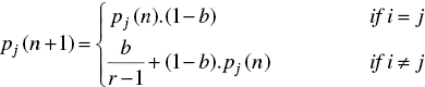
when the taken action is penalized by the environment (i.e. β(n) = 1). In the above equations, r is the number of actions. Finally, a and b denote the reward and penalty parameters and determine the amount of increases and decreases of the action probabilities, respectively. If a = b, the recurrence Eqs. (7.4) and (7.5) are called a linear reward–penalty (LR – P) algorithm, if a ≫̸ b the given equations are called linear reward–εpenalty (LR – εP ), and finally if b = 0 they are called linear reward–inaction (LR – I ). In the latter case, the action probability vectors remain unchanged when the taken action is penalized by the environment.
A learning automaton has been shown to perform well in parameter adjustment [64–66], networking [67], social networks [67], etc.
7.5 Scheduling Algorithms
One frequent feature in most of the multi‐population methods for DOPs is that the FEs are equally distributed among the sub‐populations. It implies that the same quota of the FEs is allocated to all sub‐populations, regardless of the quality of their positions in the fitness landscape. However, for several reasons, the equal distribution of FEs among sub‐populations is not a good policy [29]:
- The main goal in dynamic optimization is to locate the global optimum in a minimum amount of time and track its movements in the solution space. Therefore, strategies for quickly locating the global optimum are preferable.
- A DOP may contain several peaks (local optimum). However, as the heights of the peaks are different, they do not have the same importance from the optimality point of view. Therefore, spending an equal number of FEs on all of them postpones the process of reaching a lower error.
- Many real‐world optimization problems are large‐scale in nature. For these problems, the equal distribution of FEs among sub‐populations would be detrimental to the performance of the EC algorithms.
To alleviate the above issues, the application of SPS is presented and discussed in this chapter.
The main idea behind the SPS is to change the order by which the sub‐populations are executed with the aim to allocate more FEs to profitable sub‐populations. This in turn increases the performance of multi‐population methods in locating and tracking the optimum in dynamic environments.
The SPS methods can be roughly categorized into three classes. The first class contains strategies in which the sub‐populations are executed in a preset or random order based on their index. The second class of SPS are those methods which use one or more feedback parameters to monitor the state of the sub‐populations and choose the next sub‐population for execution, adaptively. Finally, the third class combines a preset or random SPS method with a feedback. In the rest of this section, we study eight possible SPS algorithms.
7.5.1 Round Robin SPS
The most common and simplest method for scheduling sub‐populations, which is currently used in majority of multi‐population methods, is using the round robin (RR) strategy. In this strategy, all sub‐populations are executed one by one in a circular queue (Figure 7.2). This way, FEs are equally distributed among the sub‐populations.
At each time, the sub‐population that should be executed is determined as follows:

where % is the modulo operation which returns the remainder after division of one number by another, and N is the number of sub‐populations.
7.5.2 Random SPS
The second SPS method is to execute the sub‐populations in a random manner. In this method, called random (RND) SPS, at each time, a sub‐population is chosen randomly according to the following equation:

Figure 7.2 The schematic of the round robin policy for sub‐population scheduling. Each circle represents a sup‐population.
where ![]() is the index of the sub‐population that should be executed at time t, and randi is a function that returns a random integer in the range 1 and N, and N is equal to the number of sub‐populations.
is the index of the sub‐population that should be executed at time t, and randi is a function that returns a random integer in the range 1 and N, and N is equal to the number of sub‐populations.
7.5.3 Pure‐Chance Two Action SPS
Another option for random SPS is choosing between executing the current sub‐population or executing the next sub‐population based on pure chance (PC). Let R be a random variable following the discrete uniform distribution over the set {current sub − population, next sub − population}. At each iteration, the algorithm randomly decides to execute the current sub‐population or the next sub‐population as follows:

where rand is a random number in [0, 1]. Again, N is the number of sub‐populations.
At the beginning of the optimization process, the current sub‐population is set to the first sub‐population.
7.5.4 SPS Based on Competitive Population Evaluation
As stated before, one way for scheduling the sub‐populations is based on receiving one or more feedback parameters from the search progress of the sub‐populations. The fourth SPS method, called competitive population evaluation (CPE) [42], uses the combination of the current fitness of the best individual in the sub‐populations and the amount that the error of the best individual was reduced during the previous evaluation of the sub‐populations as a feedback parameter for SPS. In this method, a performance measure ![]() is first calculated for all sub‐populations as follows:
is first calculated for all sub‐populations as follows:
In the above equation, N is the number of sub‐populations and ![]() is the improvement amount of the best individual during the previous evaluation of the sub‐population i, which is computed as:
is the improvement amount of the best individual during the previous evaluation of the sub‐population i, which is computed as:
![]() is also calculated as follows:
is also calculated as follows:

Finally, the sub‐population to be executed is selected as follows:
Regarding Eq. (7.12), at each iteration, the best‐performing sub‐population takes the FEs and evolves itself until its performance drops below that of another sub‐population, where the other one takes the FEs, and this process continues during the run. Figure 7.3 summarizes the working mechanism of CPE.
7.5.5 SPS Based on Performance Index
Another way for adaptive SPS is taking other types of feedbacks into account. In [29], the authors combined the success rate and the quality of the best solution found by the sub‐populations in a single criterion called performance index (PI). The success rate (⊖) determines the portion of improvement in the individuals of a sub‐population which is defined as:

For function maximization, the PI ψi for each sub‐population i is computed as:
where ![]() is the success rate of the sub‐population i at time t. exp is a mathematical function which returns Euler's number e raised to the power of
is the success rate of the sub‐population i at time t. exp is a mathematical function which returns Euler's number e raised to the power of ![]() , and
, and ![]() represents the fitness value of the best solution found by sub‐population i at time t.
represents the fitness value of the best solution found by sub‐population i at time t.

Figure 7.3 Sub‐population scheduling based on the competitive population evaluation.
For function minimization, one must convert the function minimization problem into a fitness maximization in which a fitness value ![]() is used. Here,
is used. Here, ![]() is the maximum value of the fitness function, while
is the maximum value of the fitness function, while ![]() is the fitness value of the best‐found position by sub‐population i.
is the fitness value of the best‐found position by sub‐population i.
The FEs at each stage are then allocated to the sub‐population with the highest PI, which is selected as follows:
It is easy to see that the best‐performing population will be the population with the highest fitness and success rate.
The pseudo code for the SPS based on the PI is shown in Figure 7.4.
7.5.6 SPS Based on VSLA
Another interesting approach for SPS is by using decision making tools like learning automata. One way to model the SPS using learning automata is by applying an N‐action VSLA, where its actions correspond to different sub‐populations, i.e. n1, n2, …, nN [29]. In order to select the next sub‐population for execution, the learning automaton LAsub − pop selects one of its actions, e.g. αi, randomly based on its action probability vector. Then, depending on the selected action, the corresponding sub‐population is executed.
After execution of the selected sub‐population, the automaton LAsub − pop updates its probability vector based on the reinforcement signal received in response to the selected action. Based on the received reinforcement signal, the automaton determines whether its action was a right or wrong, updating its probability vector accordingly. To monitor the overall progress of the SPS process, the reinforcement signal is generated as follows:

Figure 7.4 Sub‐population scheduling based on the performance index.

where f is the fitness function, and ![]() is the global best individual of the algorithm at time step t. According to Eq. (7.16), if the quality of the best‐found solution by the algorithm improves, then a favorable signal is received by the automaton LAsub − pop . Afterwards, the probability vector of the LAsub − pop is modified based on the learning algorithm of the automaton. The structure of the VLSA‐based SPS method is given in Figure 7.5.
is the global best individual of the algorithm at time step t. According to Eq. (7.16), if the quality of the best‐found solution by the algorithm improves, then a favorable signal is received by the automaton LAsub − pop . Afterwards, the probability vector of the LAsub − pop is modified based on the learning algorithm of the automaton. The structure of the VLSA‐based SPS method is given in Figure 7.5.
7.5.7 SPS Based on FSLA
Apart from the above VSLA approach, one can model the SPS with FSLA. The seventh SPS algorithm is modeled by an FSLA with N states Φ = (Φ1, Φ2, …, ΦN ), the action set α = (α1, ⋯, αN ), and the environment response β = {0, 1} which is related to reward and penalty. Figure 7.6 illustrates the state transition and action selection in the proposed model.
Initially, the automaton is in state i = 1. Therefore, the automaton selects action α1 which is related to evolving the sub‐population n1. Generally speaking, when the automaton is in state i = 1, …, N, it performs the corresponding action αi which is executing the sub‐population ni . Afterwards, the FSLA receives an input β according to Eq. (7.16). If β = 0, FSLA stays in the same state, otherwise it goes to the next state.

Figure 7.5 Sub‐population scheduling based on the variable structure learning automaton.

Figure 7.6 The schematic of the proposed FSLA for scheduling the sub‐populations. Each circle represents a state of the automaton. The symbols “U” and “F” correspond to unfavorable and favorable responses accordingly.

Figure 7.7 Sub‐population scheduling based on the fixed structure learning automaton.
Qualitatively, the simple strategy used by FSLA‐based scheduling implies that the corresponding multi‐population EC algorithm continues to execute whatever sub‐population it was evolving earlier as long as the response is favorable but changes to another sub‐population as soon as the response is unfavorable. Figure 7.7 shows the different steps of the FSLA model for SPS.
7.5.8 SPS Based on STAR Automaton
Finally, the last SPS method is based on STAR with deterministic reward and deterministic penalty [68]. The automaton can be in any of N + 1 states Φ = (Φ0, Φ1, Φ2, …, ΦN ), the action set is α = (α1, ⋯, αN ), and the environment response is β = {0, 1}, which is related to reward and penalty. The state transition and action selection are illustrated in Figure 7.8.
When the automaton is in any state i = 1, …, N, it performs the corresponding action αi which is related to evolving the sub‐population ni . On the other hand, the state Φ0 is called the “neutral” state: when in that state, the automaton chooses any of the N actions with equal probability ![]() .
.
Both reward and penalty cause deterministic state transitions, according to the following rules [68]:
- When in state Φ0 and chosen action is i (i = 1, …, N), if rewarded go to state Φi with probability 1. If punished, stay in state Φ0 with probability 1.
- When in state Φi, i ≠ 0 and chosen action is i (i = 1, …, N), if rewarded stay in state Φi with probability 1. If punished, go to state Φ0 with probability 1.
With these in mind, the STAR‐based SPS can be described as follows. At the commencement of the run, the automaton is in state Φ0. Therefore, the automaton chooses one of its actions, say αr, randomly. The action chosen by the automaton is applied to the environment, by evolving the corresponding sub‐population r, which in turn emits a reinforcement signal β according to Eq. (7.16). The automaton moves to state Φr if it has been rewarded and it stays in state Φ0 in the case of punishment. On the other hand, when in state Φi ≠ 0, the automaton chooses an action based on the current state it resides in. That is, action αi is chosen by the automaton if it is in the state Φi ≠ 0.
Figure 7.8 The schematic of the STAR for sub‐population scheduling. Each circle represents a state of the automaton. The symbols “U” and “F” correspond to unfavorable and favorable responses accordingly.
Consequently, sub‐population i is evolved. Again, the environment responds to the automaton by generating a reinforcement signal according to Eq. (7.16). On the basis of received signal β, the state of the automaton is updated. If β = 0, STAR stays in the same state, otherwise it moves to Φ0. The algorithm repeats this process until the terminating condition is satisfied. Figure 7.9 shows the details of the proposed scheduling method.
A summary of various SPS strategies is given in Table 7.1.
7.6 Application of the SPS Algorithms on a Multi‐Population Evolutionary Dynamic Optimization Method
In the following section, we describe how the mentioned SPS schemes can be incorporated into an existing multi‐population method for DOPs. Although several options exist, we have considered DynDE, the algorithm proposed in [41]. DynDE has been extensively studied in the past, showing very good results in challenging DOPs.

Figure 7.9 Sub‐population scheduling based on the STAR.
In order to describe DynDE, we will explain the DE paradigm first, which is the underlying optimization method in DynDE. Later, we give a brief overview of DynDE.
7.6.1 Differential Evolution
DE [69, 70] is a well‐known EC paradigm which is one of the most powerful stochastic real‐parameter optimization algorithms. Over the past decade, DE has gained much popularity because of its simplicity, effectiveness, and robustness.
The main idea of DE is to use spatial difference among the population of vectors to guide the search process toward the optimum solution. The rest of this section describes the main operational stages of DE in detail.
Table 7.1 Description of different SPS strategies.
| Method | Strategy | Scheduling mechanism | Feedback parameter |
| RR | Preset | All sub‐populations are executed one‐by‐one in a circular queue | — |
| RND | Random | Sub‐populations are executed in a random manner | — |
| PC | Random | Each sub‐population is either executed or skipped randomly | — |
| CPE | Adaptive | The sub‐population with the highest fitness and improvement is executed at each time | Fitness of the best individual and its fitness improvement |
| PI | Adaptive | The sub‐population with the highest fitness and success rate is executed at each time | Success rate and the quality of the best individual |
| VSLA | Adaptive | Sub‐populations are scheduled using VSLA | Success or failure of the global best individual |
| FSLA | Hybrid | Sub‐populations are scheduled using FSLA | Success or failure of the global best individual |
| STAR | Hybrid | Sub‐populations are scheduled using STAR | Success or failure of the global best individual |
7.6.1.1 Initialization of Vectors
DE starts with a population of NP randomly generated vectors in a D‐dimensional search space. Each vector i, also known as genome or chromosome, is a potential solution to an optimization problem which is represented by ![]() . The initial population of vectors is simply randomized into the boundary of the search space according to a uniform distribution as follows:
. The initial population of vectors is simply randomized into the boundary of the search space according to a uniform distribution as follows:
where iϵ[1, 2, …, NP] is the index of ith vector of the population, jϵ[1, 2, …, D] represents the jth dimension of the search space, and randj [0, 1] is a uniformly distributed random number corresponding to the jth dimension. Finally, lbj and ubj are the lower and upper bounds of the search space corresponding to the jth dimension of the search space.
7.6.1.2 Difference‐vector‐based Mutation
After initialization of the vectors in the search space, a mutation is performed on each genome i of the population to generate a donor vector ![]() corresponding to target vector
corresponding to target vector ![]() . Each component of donor vector
. Each component of donor vector ![]() , using a DE/rand/1 mutation strategy, is given by:
, using a DE/rand/1 mutation strategy, is given by:
where ![]() is the scaling factor used to control the amplification of difference vector, and r1, r2 and r3 are uniformly distributed random integers on the interval [1, NP] such that r1 ≠ r2 ≠ r3 ≠ i.
is the scaling factor used to control the amplification of difference vector, and r1, r2 and r3 are uniformly distributed random integers on the interval [1, NP] such that r1 ≠ r2 ≠ r3 ≠ i.
Different mutation strategies have been outlined in [71]. If the generated mutant vector is out of the search boundary, a repair operator is used to bring ![]() back to the feasible region.
back to the feasible region.
7.6.1.3 Crossover
To introduce diversity to the population of genomes, DE utilizes a crossover operation to combine the components of target vector ![]() and donor vector
and donor vector ![]() , to form the trial vector
, to form the trial vector ![]() . Two types of crossover are commonly used in the DE community, which are called binomial crossover and exponential crossover. Binomial crossover is the underlying crossover in DynDE which is defined as follows:
. Two types of crossover are commonly used in the DE community, which are called binomial crossover and exponential crossover. Binomial crossover is the underlying crossover in DynDE which is defined as follows:

where randij [0, 1] is a random number drawn from a uniform distribution between 0 and 1, CR ∈ (0, 1) is the crossover probability which is used to control the approximate number of components that are transferred to the trial vector. jrand is a random index in the range [1, D], which ensures the transmitting of at least one component from the donor to the trial vector.
7.6.1.4 Selection Finally, a selection approach is performed on vectors to determine which vector (![]() or
or ![]() ) should survive in the next generation. The most fitted vector is chosen to be the member of the next generation.
) should survive in the next generation. The most fitted vector is chosen to be the member of the next generation.
Different extensions of DE can be specified using the general convention DE/x/y/z, where DE stands for “Differential Evolution,” x represents a string denoting the base vector to be perturbed, y is the number of difference vectors considered for perturbation of x, and z stands for the type of crossover being used, i.e. exponential or binomial, [71]. Figure 7.10 shows a sample pseudo‐code for canonical DE.
DE has several advantages that make it a powerful tool for optimization tasks. Specifically, (i) DE has a simple structure and is easy to implement; (ii) despite its simplicity, DE exhibits a high performance; (iii) the number of control parameters in the canonical DE [69] are very few (i.e. NP, F, and CR); (iv) due to its low space complexity, DE is suitable for handling large‐scale problems.
7.6.2 DynDE
DynDE starts with a predefined number of sub‐populations, exploring the entire search space to locate the optimum. Each sub‐population is composed of normal and Brownian individuals.
Figure 7.10 Canonical differential evolution.
7.6.2.1 Normal Individuals
Normal individuals follow the principles of the DE. Although various schemes are typically used for DE, according to the authors [41], DE/best/2/bin produces the best results. In this scheme, the following mutation strategy is used:
here, ![]() are four randomly selected vectors from the sub‐population. In addition,
are four randomly selected vectors from the sub‐population. In addition, ![]() is the best vector from the sub‐population.
is the best vector from the sub‐population.
7.6.2.2 Repair Operator
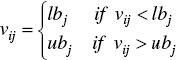
If the generated mutant vector is out of the search boundary, a repair operator is used to bring ![]() back to the feasible region. Different strategies have been proposed to repair the out of bound individuals. In this chapter, if the jth element of the ith mutant vector, i.e. vij, is out of the search region [lbj, ubj ], then it is repaired as follows:
back to the feasible region. Different strategies have been proposed to repair the out of bound individuals. In this chapter, if the jth element of the ith mutant vector, i.e. vij, is out of the search region [lbj, ubj ], then it is repaired as follows:
Afterwards, the binomial crossover is applied to form the trial vector ![]() according to Eq. (7.19).
according to Eq. (7.19).
7.6.2.3 Brownian Individuals
On the other hand, Brownian individuals are not generated according to the DE/best/2/bin scheme. They are created around the center of the best individual of the sub‐population according to the following equation:
where ![]() is a Gaussian distribution with zero mean and standard deviation σ. As shown in [41], σ = 0.2 is a suitable value for this parameter.
is a Gaussian distribution with zero mean and standard deviation σ. As shown in [41], σ = 0.2 is a suitable value for this parameter.
7.6.2.4 Exclusion
In order to prevent different sub‐populations from settling on the same peak, an exclusion operator is applied. This operator triggers when the distance between the best individuals of any two sub‐populations becomes less than the threshold rexcl, and reinitializes the worst performing sub‐population in the search space. The parameter rexcl is calculated as follows:

where X is the range of the search space for each dimension, and p is the number of existing peaks in the landscape.
7.6.2.5 Detection and Response to the Changes
Several methods have been suggested for detecting changes in dynamic environments. See for example [11] for a good survey on the topic. The most frequently used method consists in reevaluating memories of the algorithm for detecting inconsistencies in their corresponding fitness values. In DynDE the best solution of each sub‐population was considered. At the beginning of each iteration, the algorithm reevaluates these solutions and compares their current fitness values against those from the previous iteration. If at least one inconsistency is found from these comparisons, then one can assume that the environment has changed. Once a change is detected, all sub‐populations are reevaluated.
The procedure for DynDE algorithm is summarized in Figure 7.11.
Bearing in mind the inner working mechanism of DynDE, it is easy to include any SPS scheme in it.
In the rest of this chapter, DynDE with different SPS schemes is specified using the general convention DynDE‐XXX, where XXX stands for the type of SPS being used, i.e. RR, RND, etc. For example, DynDE‐RND denotes the DynDE with random SPS.
7.7 Computational Experiments
In this section, different SPS algorithms are empirically analyzed by means of computational experiments. The structure of this section is as follows: first, the technical aspects of the artificial DOP used for testing the algorithms is introduced. Then, the performance measures employed for assessing the algorithms are described. Finally, the simulation results are presented and discussed.

Figure 7.11 DynDE algorithm.
7.7.1 Dynamic Test Function
One of the most widely used dynamic test functions in the literature is the Moving Peaks Benchmark (MPB) [17]. MPB is a real‐valued dynamic environment with a D‐dimensional landscape consisting of m peaks, where the height, width, and position of each peak are changed slightly every time a change occurs in the environment [72]. Different landscapes can be defined by specifying the shape of the peaks and some other parameters. A typical peak shape is conical which is defined as follows:
where Ht (i) and Wt (i) are the height and width of peak i at time t, respectively.
In MPB, both position and objective function of the problem are subject to change. The control parameters of the MPB are φ = (H, W, X), that deviate from their current values, every time a change occurs, according to the following equation:
where ∆φ is the deviation of the control parameters, σ denotes a normally distributed random number with mean zero and standard deviation one, and φseverity is a constant number that indicates the change severity of φ. The coordinates of each dimension j ∈ [1, D] of peak i at time t are expressed by Xt (i, j), while D is the problem dimensionality. A typical change of a single peak can be modeled as follows:
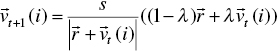
where σh and σw are two random Gaussian numbers with zero mean and standard deviation one. Moreover, the shift vector ![]() is a combination of a random vector
is a combination of a random vector ![]() , which is created by drawing random numbers in [−0.5, 0.5] for each dimension, and the current shift vector
, which is created by drawing random numbers in [−0.5, 0.5] for each dimension, and the current shift vector ![]() , and normalized to the length s. Parameter λ ∈ [0.0, 1.0] specifies the correlation of each peak's changes to the previous one. This parameter determines the trajectory of changes, where λ = 0 means that the peaks are shifted in completely random directions and λ = 1 means that the peaks always follow the same direction, until they hit the boundaries where they bounce off.
, and normalized to the length s. Parameter λ ∈ [0.0, 1.0] specifies the correlation of each peak's changes to the previous one. This parameter determines the trajectory of changes, where λ = 0 means that the peaks are shifted in completely random directions and λ = 1 means that the peaks always follow the same direction, until they hit the boundaries where they bounce off.
In this chapter we consider the so‐called Scenario 2, which is the most widely used configuration of MPB. Unless stated otherwise, the MPB's parameters are set according to the values listed in Table 7.2 (default values). In addition, to investigate the effect of the environmental parameters (i.e. the change severity, change period, number of peaks, number of dimensions) on the performance of the proposed SPS methods, various experiments were carried out with different combinations of other tested values listed in Table 7.2.
7.7.2 Performance Measure
Several criteria have been already proposed in the literature for measuring the performance of the optimization algorithms in DOPs [73]. In order to validate the efficiency of the tested SPS algorithms, we considered the offline error, which is the most well‐known metric for dynamic environments [74]. This measure [75] is defined as the average of the smallest error found by the algorithm in every time step:
where T is the maximum number of FEs so far and ![]() is the minimum error obtained by the algorithm at the time step t. We assume that a FE used by the algorithm corresponds to a single time step.
is the minimum error obtained by the algorithm at the time step t. We assume that a FE used by the algorithm corresponds to a single time step.
7.7.3 Experimental Settings
For each experiment of a SPS algorithm on a specific DOP, 50 independent runs with different random seeds were performed. Each run ends when the algorithm has consumed 500 000 FEs. The experimental results are reported in terms of average offline error and standard error, which is computed as standard deviation divided by the squared root of the number of runs.
Table 7.2 Parameter settings for the moving peaks benchmark.
| Parameter | Default values (Scenario 2) | Other tested values |
| Number of peaks (m) | 10 | 1, 2, 5, 7, 20, 30, 40, 50, 100, 200 |
| Height severity | 7.0 | |
| Width severity | 1.0 | |
| Peak function | Cone | |
| Number of dimensions (D) | 5 | 10, 15, 20, 25, 30 |
| Height range (H) | ∈[30.0, 70.0] | |
| Width range (W) | ∈ [1.0, 12.0] | |
| Standard height (I) | 50.0 | |
| Search space range (A) | [0.0, 100.0] D | |
| Frequency of change (f) | 5000 | 1000, 2000, 3000, 4000 |
| Shift severity (s) | 1 | 3, 5 |
| Correlation coefficient (λ) | 0.0 | |
| Basic function | No |
To determine the differences among tested algorithms, we applied nonparametric tests. First, we applied the Friedman's test (P < 0.05) to verify whether significant differences exist at group level, that is, among all algorithms. In the case that such differences exist, then a Wilcoxon test (α = 0.05) is applied to compare the best‐performing algorithm among DynDE‐RND, DynDE‐PC, DynDE‐CPE, DynDE‐PI, DynDE‐VSLA, DynDE‐FSLA, and DynDE‐STAR with DynDE‐RR, which is the commonly used SPS algorithm for multi‐population methods. The outcomes of the Wilcoxon test revealing that statically significant differences exist between the algorithms are highlighted with an asterisk symbol.
In addition, when reporting the results, the last column(row) of each table includes the improvement rate (%Imp) of the best‐performing DynDE variant vs. the DynDE‐RR. This measure is computed for every problem instance i as follows:

where ei, DynDE − RR is the error value obtained by DynDE‐RR for the problem i. Similarly, ei, Best is the best (minimum) offline error obtained by the other DynDE variants.
Table 7.3 Default parameter settings for DynDE and VSLA‐based sub‐population scheduling method.
| Parameter | Default value |
| Number of populations | 10 |
| Number of Brownian individuals | 2 |
| Number DE individuals | 4 |
| σ | 0.2 |
| Exclusion radius | 31.5 |
| F | 0.5 |
| CR | 0.5 |
| Reward parameter (a) | 0.15 |
| Penalty parameter (b) | 0.05 |
The parameters setting of the DynDE, and the reward and penalty factors for the VSLA‐based SPS, are as shown in Table 7.3.
In order to draw valid conclusions regarding the effect of including SPS in DynDE, we have employed the same parameter settings reported by the authors of the algorithm. Moreover, the values for reward and penalty parameters were set according to [29].
7.7.3.1 Experiment 1: Effect of Varying the Shift Severity and Change Frequency
The aim of this experiment is to investigate the performance comparison between different SPS methods on MPB's Scenario 2 with different shift lengths s ∈ {1, 3, 5} and change frequencies f ∈ {1000, 2000, 3000, 4000, 5000}. The numerical results of the different algorithms are reported in Table 7.4.
The results of the first set of experiments in Table 7.4 indicate that algorithms including the adaptive and hybrid SPS, i.e. DynDE‐PI, DynDE‐VSLA, DynDE‐FSLA, and DynDE‐STAR, reached better results in all DOPs. As can be observed in the last column of Table 7.4, the rate of improvement values of the best‐performing algorithm over the DynDE‐RR ranges from 12 to 29. Among tested scheduling algorithms, the DynDE‐FSLA achieved the best results in 8 out of 15 DOPs. As expected, best results for the fast‐changing DOPs (f = 1000) were obtained by the DynDE‐FSLA. Thanks to FSLA, DynDE‐FSLA is able to reduce the computational cost. The reason is that FSLA keeps an account of the rewards and penalties received for each action. It continues performing whatever action it was using earlier as long as it is rewarded, and switches from one action to another only when it receives a penalty. In contrast, VSLA chooses its action randomly based on the action probability vector kept over the action‐set. Therefore, it is probable that the automaton switches to another action even though it has received reward for doing the current action until the selection probability of an action converges to one.
Table 7.4 Comparison of offline error ± standard error of DynDE with different sub‐population scheduling algorithms on DOPs with D = 5, m = 10 and varying shift severities and change intervals.
| MPB | Method | ||||||||||
| s | f | DynDE‐RR | DynDE‐RND | DynDE‐PC | DynDE‐CPE | DynDE‐PI | DynDE‐VSLA | DynDE‐FSLA | DynDE‐STAR | %Imp | |
| 1 | 1000 | 3.35 ± 0.04 | 3.61 ± 0.04 | 3.82 ± 0.05 | 3.18 ± 0.03 | 2.96 ± 0.05 | 2.83 ± 0.04 | 2.76 ± 0.04 | 2.85 ± 0.04 | 17.61* | |
| 2000 | 2.31 ± 0.05 | 2.47 ± 0.05 | 2.56 ± 0.04 | 2.25 ± 0.05 | 2.05 ± 0.05 | 1.96 ± 0.04 | 1.95 ± 0.03 | 1.94 ± 0.04 | 16.01* | ||
| 3000 | 1.89 ± 0.05 | 1.97 ± 0.04 | 2.05 ± 0.04 | 1.80 ± 0.04 | 1.69 ± 0.06 | 1.65 ± 0.05 | 1.60 ± 0.04 | 1.61 ± 0.05 | 15.34* | ||
| 4000 | 1.67 ± 0.05 | 1.78 ± 0.06 | 1.80 ± 0.05 | 1.59 ± 0.04 | 1.56 ± 0.08 | 1.48 ± 0.06 | 1.49 ± 0.05 | 1.42 ± 0.04 | 14.97* | ||
| 5000 | 1.50 ± 0.05 | 1.64 ± 0.06 | 1.61 ± 0.05 | 1.49 ± 0.05 | 1.47 ± 0.08 | 1.32 ± 0.06 | 1.42 ± 0.06 | 1.31 ± 0.04 | 12.66* | ||
| 3 | 1000 | 8.19 ± 0.06 | 8.41 ± 0.06 | 8.68 ± 0.07 | 8.03 ± 0.06 | 6.44 ± 0.07 | 6.48 ± 0.05 | 6.06 ± 0.05 | 6.37 ± 0.05 | 26.00* | |
| 2000 | 5.13 ± 0.06 | 5.33 ± 0.06 | 5.44 ± 0.07 | 5.12 ± 0.06 | 4.01 ± 0.07 | 4.13 ± 0.06 | 3.90 ± 0.05 | 4.06 ± 0.05 | 23.97* | ||
| 3000 | 3.85 ± 0.07 | 4.00 ± 0.07 | 4.02 ± 0.07 | 3.77 ± 0.06 | 3.05 ± 0.08 | 3.18 ± 0.08 | 2.98 ± 0.06 | 3.08 ± 0.07 | 22.59* | ||
| 4000 | 3.14 ± 0.07 | 3.26 ± 0.07 | 3.30 ± 0.07 | 3.07 ± 0.06 | 2.52 ± 0.08 | 2.63 ± 0.07 | 2.47 ± 0.06 | 2.54 ± 0.07 | 21.33* | ||
| 5000 | 2.69 ± 0.07 | 2.82 ± 0.07 | 2.81 ± 0.06 | 2.61 ± 0.07 | 2.24 ± 0.08 | 2.23 ± 0.06 | 2.22 ± 0.06 | 2.16 ± 0.06 | 19.70* | ||
| 5 | 1000 | 13.67 ± 0.10 | 13.92 ± 0.09 | 14.20 ± 0.09 | 13.37 ± 0.09 | 10.13 ± 0.09 | 10.44 ± 0.08 | 9.59 ± 0.08 | 10.15 ± 0.08 | 29.84* | |
| 2000 | 8.66 ± 0.10 | 8.76 ± 0.09 | 8.90 ± 0.10 | 8.56 ± 0.09 | 6.13 ± 0.10 | 6.57 ± 0.09 | 6.14 ± 0.08 | 6.38 ± 0.08 | 29.21* | ||
| 3000 | 6.29 ± 0.09 | 6.39 ± 0.09 | 6.53 ± 0.10 | 6.19 ± 0.09 | 4.45 ± 0.10 | 4.88 ± 0.09 | 4.57 ± 0.08 | 4.73 ± 0.08 | 29.25* | ||
| 4000 | 4.98 ± 0.08 | 5.10 ± 0.09 | 5.14 ± 0.09 | 4.88 ± 0.07 | 3.59 ± 0.09 | 3.87 ± 0.08 | 3.61 ± 0.07 | 3.82 ± 0.08 | 27.91* | ||
| 5000 | 4.26 ± 0.10 | 4.31 ± 0.10 | 4.35 ± 0.08 | 4.18 ± 0.09 | 3.17 ± 0.10 | 3.33 ± 0.09 | 3.11 ± 0.08 | 3.24 ± 0.08 | 26.99* | ||
Best values are shown in bold.
From Table 7.4, it is clear that the SPS approach can significantly improve the performance of DynDE‐RR. It should be noted that, except for DynDE‐RND and DynDE‐PC, which act in random manners, the rest of the SPS algorithms are an improvement over the basic algorithm, i.e. DynDE‐RR. As can be inferred from Table 7.4, SPS can improve the performance of DynDE‐RR by 22.22% on average.
7.7.3.2 Experiment 2: Effect of Varying Number of Peaks
The experiment aims to investigate the performance comparison between different SPS algorithms on DOPs with different number of peaks m ϵ {1, 2, 5, 7, 10, 20, 30, 40, 50, 100, 200}. The other environmental parameters are set according to the MPB's Scenario 2 shown in Table 7.2. The obtained results are reported in Table 7.5.
For a single‐peak environment, DynDE‐FSLA is remarkably superior to the other methods. The reason lies in the fact that DynDE‐FSLA has a faster rate of convergence to the desired action. For those DOPs with m ≤ 10, best values correspond to the STAR‐based approaches, with an improvement rate ranging from 12.66 to 36.51. Finally, for DOPs with a higher number of peaks m > 10, DynDE‐PI is superior to the others. One possible explanation for such good performance can be due to combining the success rate and the quality of the local best solution into a single feedback parameter, contributing in this way to the algorithm exploration.
It is also worth noticing that when the number of peaks is high (m = 100, 200) even the random SPS, i.e. DynDE‐RND, could produce better results than DynDE‐RR.
7.7.3.3 Experiment 3: Effect of Increasing the Number of Dimensions
In this experiment, the performance of the eight SPS algorithms is investigated on the MPB with different dimensionalities D ∈ {5, 10, 15, 20, 25, 30} and the other dynamic and complexity parameters are the same as the Scenario 2 of the MPB listed in Table 7.2.
As can be clearly observed in Table 7.6, the advantage of using SPS is more marked by increasing the scale of the DOP. As the number of dimensions is increased from 10 to 30, the best rate of improvement values of the SPS methods increases monotonically. This is a further argument to confirm the effectiveness of the SPS.
In order to provide some insights about the performance of the tested algorithms over the all simulated DOPs, a graphical representation using a box plot is presented in Figure 7.12. Each boxplot in the figure corresponds to a DynDE variant with lines at the lower quartile, median as solid black line, and upper quartile data values, where the whiskers are the lines extending from each end of the box to show the extent of the rest of the data. Values outside the range of the box plot are shown as individual points.
Table 7.5 Comparison of offline error ± standard error of DynDE with different sub‐population scheduling algorithms on dynamic environments modeled with MPB.
| m | DynDE‐RR | DynDE‐RND | DynDE‐PC | DynDE‐CPE | DynDE‐PI | DynDE‐VSLA | DynDE‐FSLA | DynDE‐STAR | %Imp |
| 1 | 3.80 ± 0.17 | 4.85 ± 0.21 | 4.88 ± 0.20 | 2.79 ± 0.16 | 2.70 ± 0.11 | 3.07 ± 0.12 | 2.37 ± 0.10 | 2.49 ± 0.10 | 37.63* |
| 2 | 2.41 ± 0.17 | 2.64 ± 0.16 | 2.77 ± 0.12 | 1.93 ± 0.15 | 1.63 ± 0.13 | 1.88 ± 0.14 | 1.54 ± 0.05 | 1.53 ± 0.05 | 36.51* |
| 5 | 1.64 ± 0.09 | 1.70 ± 0.07 | 1.87 ± 0.08 | 1.55 ± 0.08 | 1.32 ± 0.09 | 1.41 ± 0.08 | 1.32 ± 0.06 | 1.30 ± 0.07 | 20.73* |
| 7 | 1.63 ± 0.08 | 1.66 ± 0.05 | 1.82 ± 0.07 | 1.59 ± 0.06 | 1.50 ± 0.09 | 1.32 ± 0.05 | 1.46 ± 0.08 | 1.32 ± 0.05 | 19.01* |
| 10 | 1.50 ± 0.05 | 1.64 ± 0.06 | 1.61 ± 0.05 | 1.49 ± 0.05 | 1.47 ± 0.08 | 1.32 ± 0.06 | 1.42 ± 0.06 | 1.31 ± 0.04 | 12.66* |
| 20 | 2.74 ± 0.07 | 2.73 ± 0.06 | 2.77 ± 0.06 | 2.66 ± 0.07 | 2.46 ± 0.08 | 2.60 ± 0.07 | 2.58 ± 0.07 | 2.54 ± 0.07 | 10.21* |
| 30 | 3.22 ± 0.10 | 3.24 ± 0.11 | 3.31 ± 0.09 | 3.25 ± 0.11 | 2.91 ± 0.11 | 3.05 ± 0.10 | 3.15 ± 0.10 | 3.02 ± 0.08 | 9.62* |
| 40 | 3.46 ± 0.08 | 3.54 ± 0.08 | 3.56 ± 0.09 | 3.53 ± 0.09 | 3.28 ± 0.09 | 3.34 ± 0.07 | 3.38 ± 0.08 | 3.41 ± 0.09 | 5.20 |
| 50 | 3.81 ± 0.10 | 3.86 ± 0.08 | 3.90 ± 0.11 | 3.77 ± 0.09 | 3.38 ± 0.10 | 3.56 ± 0.09 | 3.71 ± 0.10 | 3.62 ± 0.10 | 11.28* |
| 100 | 4.21 ± 0.12 | 4.15 ± 0.11 | 4.11 ± 0.09 | 4.15 ± 0.12 | 3.78 ± 0.11 | 3.88 ± 0.11 | 4.02 ± 0.09 | 3.97 ± 0.09 | 10.21* |
| 200 | 3.99 ± 0.12 | 3.86 ± 0.09 | 3.94 ± 0.10 | 3.98 ± 0.11 | 3.62 ± 0.09 | 3.71 ± 0.09 | 3.77 ± 0.09 | 3.71 ± 0.09 | 9.27 |
Best values are shown in bold.
Table 7.6 Average offline error ± standard error of algorithms on DOPs with m = 10, s = 1, and different dimensionalities.
| Method | Number of dimensions (D) | |||||
| 5 | 10 | 15 | 20 | 25 | 30 | |
| DynDE‐RR | 1.50 ± 0.05 | 4.41 ± 0.22 | 6.75 ± 0.23 | 9.05 ± 0.29 | 11.37 ± 0.29 | 14.30 ± 0.46 |
| DynDE‐RND | 1.64 ± 0.06 | 4.56 ± 0.24 | 7.00 ± 0.25 | 9.27 ± 0.28 | 11.75 ± 0.34 | 14.49 ± 0.45 |
| DynDE‐PC | 1.61 ± 0.05 | 4.52 ± 0.22 | 7.18 ± 0.28 | 9.26 ± 0.27 | 11.96 ± 0.35 | 14.87 ± 0.45 |
| DynDE‐CPE | 1.49 ± 0.05 | 4.25 ± 0.21 | 6.21 ± 0.23 | 8.43 ± 0.28 | 10.34 ± 0.33 | 12.93 ± 0.51 |
| DynDE‐PI | 1.47 ± 0.08 | 4.03 ± 0.23 | 5.87 ± 0.26 | 7.33 ± 0.25 | 8.90 ± 0.33 | 10.30 ± 0.36 |
| DynDE‐VSLA | 1.32 ± 0.06 | 3.99 ± 0.23 | 5.60 ± 0.25 | 6.95 ± 0.23 | 8.11 ± 0.25 | 9.43 ± 0.29 |
| DynDE‐FSLA | 1.42 ± 0.06 | 4.05 ± 0.21 | 5.60 ± 0.23 | 7.23 ± 0.23 | 8.53 ± 0.25 | 9.64 ± 0.28 |
| DynDE‐STAR | 1.31 ± 0.04 | 3.94 ± 0.22 | 5.73 ± 0.23 | 7.22 ± 0.25 | 8.29 ± 0.25 | 9.65 ± 0.30 |
| %Imp | 12.66* | 10.65* | 17.03* | 23.20* | 28.67* | 34.05* |
Best values are shown in bold.
Regarding Figure 7.12, some general observations can be made as follows:
- The boxplots for PI, VSLA, FSLA, and STAR are comparatively shorter than the other SPS methods. This suggests that PI, VSLA, FSLA, and STAR hold different performances compared to RR, RND, PC, and CPE.
- The boxplots for PI, VSLA, FSLA, and STAR are comparatively lower than RR, RND, PC, and CPE. This suggests a difference between the two groups of methods.
Moreover, Figure 7.13 shows the mean offline error of each SPS method with 95% confidence intervals for all the reported results from Table 7.4 to Table 7.6. The circles represent the mean offline error obtained by each SPS algorithm and error bars represent 95% confidence intervals for the mean. In addition, the means for every method are connected by a line. From Figure 7.13, it is observed that the results of PI, VSLA, FSLA, and STAR are significantly better than those of RR, RND, PC, CPE. Besides, while PI, VSLA, FSLA, and STAR show a similar performance, the mean error of FSLA is lower than the others.

Figure 7.12 Boxplot for the overall performance of DynDE variants with different sub‐population scheduling methods.
Finally, in order to fully support the above conclusions, we performed pairwise comparisons with the eight algorithms using the Wilcoxon's rank sum test at 0.05 level (p < 0.05) of significance using all the reported means from the previous experiments. Table 7.7 presents whether pairwise performance comparisons between the algorithms are statistically significant or not. Each result given at the Xth row (AX) and the Yth column (AY) is marked with symbols “S+,” “S‐,” “+” or “−” to indicate that the algorithm on the Xth row is significantly better than, significantly worse than, insignificantly better than, and insignificantly worse than the algorithm on the Yth column, respectively. The rightmost column of the Table 7.7 shows the mean rank of each SPS algorithm using Friedman's multiple comparisons test with p < 0.05. It is important to note that the lower the rank the better is the algorithm performance.
From Table 7.7, it is realized that a sophisticated scheduling mechanism can efficiently enhance the performance of multi‐population methods for DOPs.

Figure 7.13 Chart for mean error values of different sub‐population scheduling algorithms with 95% confidence intervals.
Table 7.7 Results of the pairwise comparisons between different sub‐population scheduling algorithms based on offline error values in all MPB's problem instances.
| RR | RND | PC | CPE | PI | VSLA | FSLA | STAR | Mean Rank | |
| RR | S+ | S+ | S‐ | S‐ | S‐ | S‐ | S‐ | 6.1000 | |
| RND | S‐ | S+ | S‐ | S‐ | S‐ | S‐ | S‐ | 6.9833 | |
| PC | S‐ | S‐ | S‐ | S‐ | S‐ | S‐ | S‐ | 7.7000 | |
| CPE | S+ | S+ | S+ | S‐ | S‐ | S‐ | S‐ | 5.2167 | |
| PI | S+ | S+ | S+ | S+ | + | − | − | 2.6000 | |
| VSLA | S+ | S+ | S+ | S+ | − | − | − | 2.8667 | |
| FSLA | S+ | S+ | S+ | S+ | + | + | + | 2.2667 | |
| STAR | S+ | S+ | S+ | S+ | + | + | − | 2.2667 |
7.7.3.4 Experiment 4: Comparison with Other Methods from the Literature
In this experiment, we study the performance of different DynDE variants in comparison with several well‐known algorithms taken from the literature. The algorithms considered include: mQSO [23], SPSO [51], CESO [46], AmQSO [56], CellularPSO [25], ESCA [47], HmSO [26], CellularDE [30], and DynPopDE [59]. Table 7.8 shows the numerical results of different algorithms on MPB scenario 2.
Table 7.8 Comparison of offline error of different algorithms for dynamic environments modeled with MPB (Scenario 2).
| Method | Result |
| mQSO | 1.77 ± 0.05 |
| SPSO | 2.51 ± 0.09 |
| CESO | 1.38 ± 0.02 |
| AmQSO | 1.64 ± 0.05 |
| Cellular PSO | 1.93 ± 0.08 |
| ESCA | 1.53 ± 0.01 |
| HmSO | 1.47 ± 0.04 |
| CellularDE | 1.64 ± 0.03 |
| DynPopDE | 1.39 ± 0.07 |
| DynDE‐PI | 1.47 ± 0.08 |
| DynDE‐VSLA | 1.32 ± 0.06 |
| DynDE‐FSLA | 1.42 ± 0.06 |
| DynDE‐STAR | 1.31 ± 0.04 |
As can be observed in Table 7.8, DynDE‐STAR is the best‐performing method. Moreover, despite their simplicity, DynDE variants with SPS display a better or competitive performance compared with other representative multi‐population approaches.
From the analysis of the above experiments, we can reach to the conclusion that the SPS algorithm is a fairly simple scheme that can effectively improve the performance of multi‐population methods for DOPs.
7.8 Conclusions
This chapter investigates the application of scheduling to improve the performance of evolutionary multi‐population approaches in dynamic environments. Eight SPS schemes are integrated into DynDE to address DOPs. Based on dynamic test environments generated by MPB, an experimental study was carried out to test the SPS methods. From the experimental results, the following conclusions can be drawn. First, sophisticated SPS methods are efficient to improve the performance multi‐population algorithms in dynamic environments. Second, the performance of DynDE with SPS is directly affected by the selected scheduling strategy and feedback parameters.
The work studied in this chapter can be further extended in several directions. Developing other mechanisms for SPS would be an interesting direction for future work. Studying the effect of different feedback parameters in adaptive or hybrid SPS is also interesting. Evaluating the SPS for noisy dynamic environments is another future work. Finally, it is also very valuable to apply the proposed approach to several real‐world dynamic problems.
Acknowledgments
We would like to thank the editors for the invitation to participate in this book. The first author would like to express gratitude to his beloved wife Mahsa Azadeh for being an endless source of happiness, inspiration, support, and peace.
References
- 1 Shirali, A., Kazemi Kordestani, J., and Meybodi, M.R. (2018). Self‐adaptive multi‐population genetic algorithms for dynamic resource allocation in shared hosting platforms. Genet. Program Evolvable Mach. 19 (4): 505–534.
- 2 Mavrovouniotis, M. and Yang, S. (2013). Ant colony optimization with immigrants schemes for the dynamic travelling salesman problem with traffic factors. Appl. Soft Comput. 13 (10): 4023–4037.
- 3 Yang, S., Cheng, H., and Wang, F. (2010). Genetic algorithms with immigrants and memory schemes for dynamic shortest path routing problems in mobile ad hoc networks. IEEE Trans. Syst. Man Cybern. Part C Appl. Rev. 40 (1): 52–63.
- 4 Mack, Y., Goel, T., Shyy, W., and Haftka, R. (2007). Surrogate model‐based optimization framework: a case study in aerospace design. In: Evolutionary Computation in Dynamic and Uncertain Environments (eds. S. Yang, Y.‐S. Ong and Y. Jin), 323–342. Berlin, Heidelberg: Springer.
- 5 Michalewicz, Z., Schmidt, M., Michalewicz, M., and Chiriac, C. (2007). Adaptive business intelligence: three case studies. In: Evolutionary Computation in Dynamic and Uncertain Environments (eds. S. Yang, Y.‐S. Ong and Y. Jin), 179–196. Berlin, Heidelberg: Springer.
- 6 Pillac, V., Gendreau, M., Guéret, C., and Medaglia, A.L. (2013). A review of dynamic vehicle routing problems. Eur. J. Oper. Res. 225 (1): 1–11.
- 7 Hossain, M.A. and Ferdous, I. (2015). Autonomous robot path planning in dynamic environment using a new optimization technique inspired by bacterial foraging technique. Robot. Auton. Syst. 64: 137–141.
- 8 Tang, W.J., Li, M.S., Wu, Q.H., and Saunders, J.R. (2008). Bacterial foraging algorithm for optimal power flow in dynamic environments. IEEE Trans. Circuits Syst. Regul. Pap. 55 (8): 2433–2442.
- 9Sesum, V.‐C., and Kuhn, E. (2010). Applying swarm intelligence algorithms for dynamic load balancing to a cloud based call center. 2010 Fourth IEEE Int. Conf. Self‐Adapt. Self‐Organ. Syst., 255–256.
- 10 Liu, L. and Ranji Ranjithan, S. (2010). An adaptive optimization technique for dynamic environments. Eng. Appl. Artif. Intell. 23 (5): 772–779.
- 11 Nguyen, T.T., Yang, S., and Branke, J. (2012). Evolutionary dynamic optimization: a survey of the state of the art. Swarm Evol. Comput. 6: 1–24.
- 12 Hu, X. and Eberhart, R.C. (2002). Adaptive particle swarm optimization: detection and response to dynamic systems. Proc. IEEE Congr. Evol. Comput. 2: 1666–1670.
- 13 Vavak, F., Jukes, K.A., and Fogarty, T.C. (1998). Performance of a genetic algorithm with variable local search range relative to frequency of the environmental changes. Genet. Program., 22–25.
- 14 Vavak, F., Jukes, K., and Fogarty, T.C. (1997). Learning the local search range for genetic optimisation in nonstationary environments. 1997 IEEE Int. Conf. On Evol. Comput., 355–360.
- 15 Janson, S. and Middendorf, M. (2006). A hierarchical particle swarm optimizer for noisy and dynamic environments. Genet. Program Evolvable Mach. 7 (4): 329–354.
- 16 Mori, N., Kita, H., and Nishikawa, Y. (2001). Adaptation to changing environments by means of the memory based thermodynamical genetic algorithm. Trans. Inst. Syst. Control Inf. Eng. 14: 33–41.
- 17 Branke, J. (1999). Memory enhanced evolutionary algorithms for changing optimization problems. Proc. Congr. Evol. Comput., 3: 1875–1882.
- 18 Wang, H., Wang, D., and Yang, S. (2007). Triggered memory‐based swarm optimization in dynamic environments. In: Applications of Evolutionary Computing (ed. M. Giacobini), 637–646. Berlin, Heidelberg: Springer.
- 19 Hatzakis, I. and Wallace, D. (2006). Dynamic multi‐objective optimization with evolutionary algorithms: a forward‐looking approach. Proc. Genet. Evol. Comput. Conf., 1201–1208.
- 20 Rossi, C., Abderrahim, M., and Díaz, J.C. (2008). Tracking moving optima using kalman‐based predictions. Evol. Comput. 16 (1): 1–30.
- 21 Grefenstette, J.J. (1999). Evolvability in dynamic fitness landscapes: a genetic algorithm approach. Proc. IEEE Congr. Evol. Comput., 3: 1–2038.
- 22 Novoa‐Hernández, P., Corona, C.C., and Pelta, D.A. (2016). Self‐adaptation in dynamic environments – a survey and open issues. Int. J. Bio‐Inspired Comput. 8 (1): 1–13.
- 23 Blackwell, T.M. and Branke, J. (2006). Multiswarms, exclusion, and anti‐convergence in dynamic environments. IEEE Trans. Evol. Comput. 10 (4): 459–472.
- 24 Hashemi, A.B. and Meybodi, M.R. (2009). A multi‐role cellular PSO for dynamic environments. Proc. 14th Int. CSI Comput. Conf., 412–417.
- 25Hashemi, A.B. and Meybodi, M.R. (2009). Cellular PSO: A PSO for dynamic environments. 4th International Symposium on Intelligence Computation and Applications, 422–433.
- 26 Kamosi, M., Hashemi, A.B., and Meybodi, M.R. (2010). A hibernating multi‐swarm optimization algorithm for dynamic environments. Proc. Second World Congr. Nat. Biol. Inspired Comput., 363–369.
- 27 Kamosi, M., Hashemi, A.B., and Meybodi, M.R. (2010). A new particle swarm optimization algorithm for dynamic environments. Proceedings of the First International Conference on Swarm, Evolutionary, and Memetic Computing, 129–138.
- 28 Kordestani, J.K., Firouzjaee, H.A., and Reza Meybodi, M. (2018). An adaptive bi‐flight cuckoo search with variable nests for continuous dynamic optimization problems. Appl. Intell. 48 (1): 97–117.
- 29 Kordestani, J.K., Ranginkaman, A.E., Meybodi, M.R., and Novoa‐Hernández, P. (2019). A novel framework for improving multi‐population algorithms for dynamic optimization problems: a scheduling approach. Swarm Evol. Comput. 44: 788–805.
- 30 Noroozi, V., Hashemi, A.B., and Meybodi, M.R. (2011). CellularDE: A cellular based differential evolution for dynamic optimization problems. Proceedings of the 10th International Conference on Adaptive and Natural Computing Algorithms, 340–349.
- 31 Noroozi, V., Hashemi, A.B., and Meybodi, M.R. (2012). Alpinist CellularDE: A cellular based optimization algorithm for dynamic environments. Proc. Genet. Evol. Comput. Conf., 1519–1520.
- 32 Sharifi, A., Noroozi, V., Bashiri, M. et al. (2012). Two phased cellular PSO: A new collaborative cellular algorithm for optimization in dynamic environments. Proc. IEEE Congr. Evol. Comput., 1–8.
- 33 Sharifi, A., Kazemi Kordestani, J., Mahdaviani, M., and Meybodi, M.R. (2015). A novel hybrid adaptive collaborative approach based on particle swarm optimization and local search for dynamic optimization problems. Appl. Soft Comput. 32: 432–448.
- 34 Yang, S. and Li, C. (2008). Fast multi‐swarm optimization for dynamic optimization problems. Proceeding Fourth Int. Conf. Nat. Comput., 7: 624–628.
- 35 Yang, S. and Li, C. (2010). A clustering particle swarm optimizer for locating and tracking multiple optima in dynamic environments. IEEE Trans. Evol. Comput. 14 (6): 959–974.
- 36 Li, C., Nguyen, T.T., Yang, M. et al. (2015). Multi‐population methods in unconstrained continuous dynamic environments: the challenges. Inf. Sci. 296: 95–118.
- 37 Blackwell, T. and Branke, J. (2004). Multi‐swarm optimization in dynamic environments. Appl. Evol. Comput., 489–500.
- 38Trojanowski, K. (2008). Tuning quantum multi‐swarm optimization for dynamic tasks. Artif. Intell. Soft Comput. – ICAISC 2008, 499–510.
- 39 Trojanowski, K. (2008). Adaptive non‐uniform distribution of quantum particles in mQSO. Simulated Evolution and Learning: 7th International Conference, SEAL 2008, Melbourne, Australia, 7–10 December. (eds. Li, X., Kirley, M., Zhang, M. et al.), Springer Berlin Heidelberg, Berlin, Heidelberg: 91–100.
- 40 del Amo, I.G., Pelta, D.A., González, J.R., and Novoa, P. (2009). An analysis of particle properties on a multi‐swarm pso for dynamic optimization problems. Conf. Span. Assoc. Artif. Intell., 32–41.
- 41 Mendes, R. and Mohais, A.S. (2005). DynDE: A differential evolution for dynamic optimization problems. Proc. IEEE Congr. Evol. Comput., 3: 2808–2815.
- 42 du Plessis, M.C. and Engelbrecht, A.P. (2012). Using competitive population evaluation in a differential evolution algorithm for dynamic environments. Eur. J. Oper. Res. 218 (1): 7–20.
- 43 Xiao, L. and Zuo, X. (2012). Multi‐DEPSO: A DE and PSO based hybrid algorithm in dynamic environments. 1–7.
- 44 Novoa‐Hernández, P., Corona, C.C., and Pelta, D.A. (2011). Efficient multi‐swarm PSO algorithms for dynamic environments. Memetic Comput. 3 (3): 163.
- 45 du Plessis, M.C. and Engelbrecht, A.P. (2008). Improved differential evolution for dynamic optimization problems. 2008 IEEE Congr. Evol. Comput. IEEE World Congr. Comput. Intell., 229–234.
- 46 Lung, R.I. and Dumitrescu, D. (2007). A new collaborative evolutionary‐swarm optimization technique. Proc. 9th Annu. Conf. Companion Genet. Evol. Comput., 2817–2820.
- 47 Lung, R.I. and Dumitrescu, D. (2009). Evolutionary swarm cooperative optimization in dynamic environments. Nat. Comput. 9 (1): 83–94.
- 48 Kordestani, J.K., Rezvanian, A., and Meybodi, M.R. (2014). CDEPSO: a bi‐population hybrid approach for dynamic optimization problems. Appl. Intell. 40 (4): 682–694.
- 49 Branke, J., Kaussler, T., Smidt, C., and Schmeck, H. (2000). A multi‐population approach to dynamic optimization problems. In: Evolutionary Design and Manufacture (ed. I.C. Parmee), 299–307. London: Springer.
- 50 Yazdani, D., Nasiri, B., Sepas‐Moghaddam, A., and Meybodi, M.R. (2013). A novel multi‐swarm algorithm for optimization in dynamic environments based on particle swarm optimization. Appl. Soft Comput. 13 (4): 2144–2158.
- 51 Parrott, D. and Li, X. (2006). Locating and tracking multiple dynamic optima by a particle swarm model using speciation. IEEE Trans. Evol. Comput. 10 (4): 440–458.
- 52 Bird, S. and Li, X. (2007). Using regression to improve local convergence. 2007 IEEE Congr. Evol. Comput., 592–599.
- 53Li, C. and Yang, S. (2012). A general framework of multipopulation methods with clustering in undetectable dynamic environments. IEEE Trans. Evol. Comput. 16 (4): 556–577.
- 54 Nickabadi, A., Ebadzadeh, M.M., and Safabakhsh, R. (2012). A competitive clustering particle swarm optimizer for dynamic optimization problems. Swarm Intell. 6 (3): 177–206.
- 55 Halder, U., Das, S., and Maity, D. (2013). A cluster‐based differential evolution algorithm with external archive for optimization in dynamic environments. IEEE Trans. Cybern. 43 (3): 881–897.
- 56 Blackwell, T. (2007). Particle swarm optimization in dynamic environments. In: Evolutionary Computation in Dynamic and Uncertain Environments (eds. S. Yang, Y.‐S. Ong and Y. Jin), 29–49. Berlin, Heidelberg: Springer.
- 57 Yazdani, D., Akbarzadeh‐Totonchi, M.R., Nasiri, B., and Meybodi, M.R. (2012). A new artificial fish swarm algorithm for dynamic optimization problems. IEEE Congr. Evol. Comput., 1–8.
- 58 Fouladgar, N. and Lotfi, S. (2015). A novel approach for optimization in dynamic environments based on modified cuckoo search algorithm. Soft. Comput. 7: 2889–2903.
- 59 du Plessis, M.C. and Engelbrecht, A.P. (2013). Differential evolution for dynamic environments with unknown numbers of optima. J. Glob. Optim. 55 (1): 73–99.
- 60 Li, C., Nguyen, T.T., Yang, M. et al. (2016). An adaptive multipopulation framework for locating and tracking multiple optima. IEEE Trans. Evol. Comput. 20 (4): 590–605.
- 61 Li, C., Yang, S., Nguyen, T. et al. (2008). Benchmark generator for CEC 2009 competition on dynamic optimization. Technical Report, Department of Computer Science, University of Leicester.
- 62 Narendra, K.S. and Thathachar, M.A. (1974). Learning automata‐a survey. IEEE Trans. Syst. Man Cybern. 4 (4): 323–334.
- 63 Narendra, K.S. and Thathachar, M.A. (2012). Learning Automata: An Introduction. Courier Corporation.
- 64 Abedi Firouzjaee, H., Kordestani, J.K., and Meybodi, M.R. (2017). Cuckoo search with composite flight operator for numerical optimization problems and its application in tunnelling. Eng. Optim. 49 (4): 597–616.
- 65 Kordestani, J.K., Ahmadi, A., and Meybodi, M.R. (2014). An improved differential evolution algorithm using learning automata and population topologies. Appl. Intell. 41 (4): 1150–1169.
- 66 Mahdaviani, M., Kordestani, J.K., Rezvanian, A., and Meybodi, M.R. (2015). LADE: learning automata based differential evolution. Int. J. Artif. Intell. Tools 24 (6): 1550023.
- 67 Rezvanian, A., Saghiri, A.M., Vahidipour, S.M. et al. (2018). Recent Advances in Learning Automata. Berlin: Springer.
- 68Economides, A.A. and Kehagias, A. (2002). The STAR automaton: expediency and optimality properties. IEEE Trans. Syst. Man Cybern. B Cybern. 32 (6): 723–737.
- 69 Storn, R. and Price, K. (1997). Differential evolution ‐ a simple and efficient heuristic for global optimization over continuous spaces. J. Glob. Optim. 11 (4): 341–359.
- 70 Storn, R. and Price, K. (1995). Differential evolution‐a simple and efficient adaptive scheme for global optimization over continuous spaces.
- 71 Das, S. and Suganthan, P.N. (2011). Differential evolution: a survey of the state‐of‐the‐art. IEEE Trans. Evol. Comput. 15 (1): 4–31.
- 72 Branke, J. (2002). Evolutionary Optimization in Dynamic Environments. Springer Science and Business Media.
- 73 Kordestani, J.K., Rezvanian, A., and Meybodi, M.R. (2017). New measures for comparing optimization algorithms on dynamic optimization problems. Nat. Comput. 18 (4): 705–720.
- 74 Cruz, C., González, J.R., and Pelta, D.A. (2011). Optimization in dynamic environments: a survey on problems, methods and measures. Soft. Comput. 15 (7): 1427–1448.
- 75 Branke, J. and Schmeck, H. (2003). Designing evolutionary algorithms for dynamic optimization problems. In: Advances in Evolutionary Computing: Theory and Applications (eds. A. Ghosh and S. Shigeyoshi), 239–262. Berlin, Heidelberg: Springer.