
3
Advanced Ant Colony Optimization in Healthcare Scheduling
Reza Behmanesh1, Iman Rahimi1, Mostafa Zandieh2, and Amir H. Gandomi3
1 Young Researchers and Elite Club, Isfahan (Khorasgan) Branch, Islamic Azad University, Isfahan, Iran
2 Department of Industrial Management, Management and Accounting Faculty, Shahid Beheshti University, G.C., Tehran, Iran
3 Faculty of Engineering and IT, University of Technology Sydney, Ultimo, Australia
3.1 History of Ant Colony Optimization
3.1.1 Introduction to Ant Colony Optimization
The first ant colony optimization (ACO) algorithm, ant system (AS), was introduced by [1] as an optimizer, learning, natural algorithm and meta‐heuristic; and also it was applied to tackle the Traveling Salesman Problem (TSP) by [2]. It must be noted that the researcher introduced the basic algorithm and some extended versions of the basic method in his dissertation in 1992. This algorithm was designed to find an optimized route or vertices through the graph according to an ant's behavior between the nest and food resource. Since this method is inspired by the nature of ant colony behavior, it is categorized by bio‐inspired computation methods to solve problems. In nature, the ants move from their nest to find food along a random path. While moving along the route, the ants secrete pheromone on the way back. The smell of the pheromone helps other ants to tail the path for finding food. The pheromone is liquid, and it will evaporate after a short time, but more pheromone on the shorter routes remains and more ants are attracted by sniffing, and as a consequence, the ant colony on short routes is higher than on long routes because more pheromone is trailed before evaporation.
To continue, we categorize some essential and basic characteristics of ACO to ascertain this methodology. ACO includes the following special components:
- This approach is a metaheuristic algorithm.
- This method is classified as a stochastic local search (SLS) method.
- ACO is inspired by an ant's behavior in the colony, and so this is classified as a biologically‐inspired algorithm.
- ACO is a population‐based method because the algorithm applies a swarm of ants to find the objective.
- The algorithm's strategy for finding a solution is constructive, i.e. decision variables of the problem are constructed in each iteration, and it is different from the strategy of other meta‐heuristic algorithms such as genetic algorithms, which use an improvement.
- ACO is a prominent swarm intelligence technique because the passed path by each ant helps to improve the objective function in the next iteration.
On the other hand, the ACO is missing some characteristics:
- It is not a single algorithm.
- It is not an evolutionary algorithm, because there is no evolution path in the ACO approach.
- It is not a model of the behavior of real ants in nature, because the equations of ACO have been extracted according to pheromone trail foraging and probability rules. These formulations are not by nature exactly the same as an ant's movement, which passes along the shortest path.
3.1.2 The Nature of Ants' Behavior in a Colony
As stated previously, ACO was inspired by the movement of swarm ants from the nest to the food resource. In other words, it was inspired by the indirect communication of some ant species through pheromone trails. All ants secrete pheromone when coming back from a food resource to the nest. Each ant forages the higher probability paths that are determined by stronger pheromone concentrations. It was demonstrated that a big swarm of ants passes along the shortest path to find food. It was experienced by [3] in a double bridge experiment, and therefore they indicate that more ants choose the shortest path to find food. This famous experiment is indicated in Figure 3.1 and [3] presented a stochastic model and confirmed it by simulation as follows:

Figure 3.1 Double bridge experiment.
Where, Pi, b denotes the probability of choosing branch #b when ant #i decides to choose and τi, b denotes pheromone concentration corresponding to ant #i in branch #b.
As it was notated, real ants pass the shortest way between nest and food, so they solve the shortest path problem. However, artificial ants in swarm intelligence problems are taken into account as stochastic solution construction procedures, which can be considered as a searcher on a construction graph network, as indicated in Figure 3.2.
Artificial ants’ constructed paths (solutions) are based on segregated pheromone probabilistically and then these ants record the solutions in memory. Therefore, an artificial memory is built to be applied in the next iterations. These artificial ants deposit pheromones on the path that they walk on. It is possible that the pheromone evaporates after some time. Finally, the paths represent better solutions that have more pheromone trails.

Figure 3.2 Artificial ants searching on a graph.
3.2 Introduction to ACO as a Metaheuristic
3.2.1 Ant Colony Optimization Approach
This approach consists of two substantial parts. The first is to construct the solution with a probability rule and the second is to update the pheromone in order to search for better solutions. Artificial ants construct routes (solutions) probabilistically by pheromones, and these memorize the solution. On the other hand, agents secrete pheromone on the route and as a consequence there is more pheromone on the routes that present better solutions. The first ACO is called AS, in which each ant (agent) with tag #k builds a complete tour (a solution) in the grap h iteratively, and from the last visited node i chooses an unvisited node j to visit next (Figure 3.3).
It is noted that unvisited nodes are feasible neighborhood (![]() ). The probability of choosing node j after node i by ant k is determined as shown in the following equation (probabilistic choice rule):
). The probability of choosing node j after node i by ant k is determined as shown in the following equation (probabilistic choice rule):

Where τij (t) notates pheromone information that changes in any iteration, μij is heuristic information, which corresponds to the problem, α controls the relative importance of pheromone, and β controls the relative importance of heuristic information. In the second part, the pheromone trail updating strategies are presented. The pheromone update procedure in AS is formulated as follows:

Figure 3.3 Probability of choosing a model by ant k.
where sk is the solution of the kth ant and f(sk ) is its cost function. It is notated by Lk in some literature, which means it found the tour's length by ant k.
The pseudo code of ACO is presented in Figure 3.4, in which the stages of the algorithm are articulated.
For example, the AS algorithm is applied to solve TSP for the first time by [2], and we describe details of the algorithm as follows:
- The ants are set on nodes (cities) randomly so that each agent memorizes the path recorded (Figure 3.5). In other words, a solution consisting of all decision variables is saved in the memory of agent. As indicated in Figure 3.6, there are five cities and the matrix of D denotes the distances between all cities. On the other hand, a graph with prime pheromone is constructed.
- As indicated in Figure 3.6, ant #1 has several choices (C, E, D, and B) and according to transition rule Eq. (3.2), the probability choosing is determined and the ant can move to the next node (city). If setting ants on each city is done to construct the first partial solution (a decision variable of completed solution) in Figure 3.6, this stage can be repeated to the complete solution that is shown in Figure 3.7.
Figure 3.4 Pseudo code of ant colony optimization.

Figure 3.5 Inputting an instance and initializing prime pheromone.

Figure 3.6 Setting ants on cities.
Figure 3.7 Moving ants and completing solution.
- After obtaining a solution for each agent, the length of tour for each ant is calculated, and then the segregated pheromone value of the arcs (the path between two cities) is evaluated based on Eq. (3.4). Finally, the pheromone value of each arc is updated according to the second part of Eq. (3.3). The results are displayed in Figure 3.8. For example, we can observe that ants #4 and #5 passed the arc AB and deposited pheromone on this arc. Thus, for assessing the pheromone value of arc AB, only ants #4 and #5 are involved in calculating the increased pheromone. It must be noted that there is no difference between AB or BA, i.e. the reverse path for updating the pheromone value in the path. As shown in the graph, some arcs are colored, which means agent tags inside parentheses update the pheromone value of these arcs. For example, the pheromone of arc BC or CB is updated by ants #(2, 3, 4, 5).

Figure 3.8 Updating pheromone trail value for paths between cities.
- Repeat stages 1 to 3 until termination conditions are met, or the algorithm reaches the convergent condition.
3.2.2 Intensification and Diversification Mechanism in ACO
As we know, there are two major components in the literature of metaheuristic algorithms: intensification and diversification, known as exploitation and exploration [4, 5]. To make a qualified and robust algorithm metaheuristic, a balanced and adjusted combination of the exploration and exploitation mechanism is vitally important because their strategies are in contradiction with each other [6].
A good diversification or exploration strategy guarantees that an algorithm can search as many regions as possible inside the solution space in an efficient manner. Moreover, this component prevents premature convergence or being trapped in local optima, and, as a consequence, the stronger diversification leads to a slowdown in the convergence of the algorithm since this strategy implements randomization or stochastic procedures in the algorithm and the weaker exploration leads to premature convergence. In the first term of the transition rule equation of ACO, i.e. the pheromone‐based probability of choosing a node, the diversification is focused. So, more alpha as an important factor of pheromone information as well as more beta as an essential factor of heuristic information results in less exploration and more exploitation (sometimes premature convergence) in the algorithm according to the example shown in Figure 3.9. On the other hand, fewer α as well as fewer β leads to increased diversification and randomness in the search process. As indicated in Figure 3.9, when alpha is increased only node #3 is more probable to be chosen, so this path is bold, and the probability of choosing other paths (#1 and #2) is decreased.

Figure 3.9 Compare two probabilities of choosing nodes for alpha = 1 and alpha = 2.
On the other hand, the proper intensification or exploitation strategy makes sure that the algorithm exploits the experience of the search process and always intensifies the solution found to reduce randomness in the search process, then it can speed up convergence of the algorithm when the algorithm needs to decrease exploration. Therefore, the stronger intensification leads to local traps and premature convergence of the algorithm and provides meaningless solutions. Moreover, the weaker exploitation leads to a slowdown in the convergence of the algorithm.
To summarize, alpha and beta coefficients are important parameters in exploration and exploitation and need to be set to improve the performance of ACO algorithms for a specific problem.
3.3 Other Advanced Ant Colony Optimization
The first ACO algorithm, AS, was shown to be a viable approach for solving hard optimization problems; however, its performance is rather poor for large instance problems like TSP in comparison to other metaheuristics. To achieve better performance than AS, more studies were conducted to build an improved AS. There are several versions of advanced ACO that improve solution quality, and these new algorithms are extended by introducing a different pheromone update strategy or a hybrid ACO using other methods or operations. A brief list of extended new ACO algorithms is shown in Table 3.1.
Table 3.1 All versions of ACO.
| Class | ACO Algorithm | Researched by | Date |
| Pheromone update strategy‐based method | Ant System (AS) | [1] | 1991 |
| Elitist Ant System (EAS) | [7] | 1992 | |
| Ant Colony System (ACS) | [2] | 1996 | |
| Rank‐based Ant System (RBAS) | [8] | 1997 | |
| Max‐Min Ant System (MMAS) | [9] | 2000 | |
| Hybrid ACO methods | Best‐Worst Ant System (BWAS) | [10] | 2000 |
| Population‐based ACO (P‐ACO) | [11] | 2002 | |
| Beam‐ACO (BACO) | [12] | 2004 | |
| Two‐level ACO | [13] | 2015 | |
| Improved Auto‐control ACO with lazy ant (IAACO) | [14] | 2016 |
3.3.1 Elitism Ant System
In all developments over AS, the pheromone trail updating strategy was extended to improve the algorithm's performance. A first improvement, namely ASe (elitism strategy for AS) was developed by [7], where the global best solution (sgb) is considered to update the trails and the pheromone update procedure is formulated as follows:
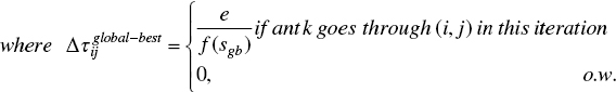
where e is the number of elitist ants and f(sgb ) is the solution cost of the best ant that is used to update arcs after each iteration.
3.3.2 Ant Colony System
The next improvement over AS is called ant colony system (ACS), which was introduced by [2]. ACS works according to a pseudo‐random proportional choice rule using a controller parameter, namely q0 . Agent #k chooses node j after node i with probability less than or equal to q0 based on the following equation (greedy walking):
On the other hand, agent #k chooses node j after node i with probability higher than q0 based on an equation that pertains to the probabilistic choice rule of AS (Eq. 3.2).
There are two pheromone updating strategies in ACS, a global pheromone update and a local pheromone update. In the global update or exploitation strategy, a single ant is used, i.e. either the global‐best ant so far or the iteration‐best is taken into account to update as follows:
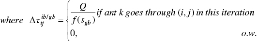
where ib refers to iteration‐best, and gb refers to global‐best ant. And in the local update or exploration strategy, ant #k decreases the pheromone when it adds a component cij to its partial solution in accordance with the following:
where parameter γ controls the exploration factor and the initial pheromone (small constant value) is notated by τ0.
3.3.3 Rank‐Based AS
Rank‐based AS (ASrank) is another version of AS that was extended by [8]. A fixed number of better ants in the current iteration are ranked, and then the global‐best ant is allowed to update trails of ranked solutions. For example, if the fixed number equals 10, it means that 10 better ants in the current iteration are ranked, and then the global‐best ant is allowed to update the pheromone trails of the ranked ant's paths.
3.3.4 Max‐Min AS
[9] developed the Max‐Min ant system (MMAS) so that only a single ant is applied to update the pheromone trail when the iteration is passed. The updating rule of MMAS is similar to ACS but there are important requirements in MMAS that should be fulfilled:
- After the iteration, only one single ant adds the pheromone value to exploit the best solutions found during iteration or the run of the algorithm.
- An interval distance trail [τmin, τmax] is considered and updated for the range of possible trails on each solution component.
- Also, pheromone trails are initialized to τmax to achieve good diversification at the beginning of the algorithm. Pheromone update strategy is according to the following equation:
(3.11)
 (3.12)
As stated, this approach applies the global‐best solution found ever from the beginning of the trial (global‐best ant) or the current iteration‐best solution (iteration‐best ant) so that both strategies are suggested. Moreover, limitations for lower and upper pheromone are written as follows:
Ibanez comments that it would be better if the pheromone were set to prime pheromone after some iterations and that this prevents premature convergence and other solutions are found and the exploration strategy is strengthened.
3.3.4 Best‐Worst AS
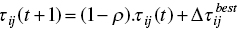
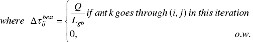
In another study, Cordón et al. [15] applied a new pheromone trail strategy along with evolutionary algorithm concepts to improve the performance of AS. First, they proposed the best‐worst performance update rule, which is based on population‐based incremental learning (PBIL). According to this strategy, edges present in global‐best ant are updated as follows:

and pheromone deposited based on a global‐best solution (sgb ).
Then, edges present in the worst current ant are penalized in the evaporation rule:
where siw is the worst solution in each iteration.
Finally, some random pheromone trails are mutated to make more exploration in the search method, as done in PBIL. According to this rule, each row of the pheromone matrix is mutated with probability Pm, as follows:
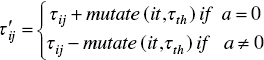
where a is a random value in {0,1}, it is a current iteration, and τth is the mean of pheromone trail in edges that are generated by global‐best.
3.3.5 Population‐Based ACO
In a population‐based ACO (P‐ACO) proposed by [11], the population‐based concepts were the inspiration, and the basic ACO is developed to a new high‐quality algorithm considering the population set to solve dynamic optimization problems. First, the empty set of population, namely P, is saved such that its capacity equals the number of ants, i.e. k. In the current iteration, the best ant updates the pheromone trail matrix similar to the Max‐Min AS performance, in which pheromone addition is according to the best solution ever found by the best ant; however, the evaporation or pheromone decrease is not done by ants, and then it enters the population set till the kth generation.
When the P set is full of the best ants obtained from all k iterations, for generation k + 1 and m ore, the best ant of the iteration is replaced with one of the ants inside the population according to update strategies defined in the next section. Therefore, that ant is removed from the population and the best enters the population. Instea of decrasing pheromone value based on an evaporation rule, a new method is introduced, in which the removed ant decreases the pheromone matrix according to its pheromone value, i.e. the same value that it added to the pheromone matrix when it entered to the population as follows:
The pseudo code of population‐based ACO is presented in Figure 3.10, in which the stages of the algorithm are coded.

Figure 3.10 Pseudo code of population‐based ant colony optimization.
The researchers defined several population pheromone update strategies in other research [16] that is briefed below:
- Age of ant: in this strategy, the oldest ant of the population (the ant that is entered to the population in the oldest iteration) leaves the population, and the newest solution is entered. This strategy is called age‐based strategy or was referred to as FIFO‐Queue by researchers in a previous paper [11].
- Quality: If the candidate solution of the current iteration is better than the worst solution inside P set, the former replaces the latter in P. Otherwise, P set does not change.
- Elitism: This strategy considered inserting an ant into the population set, but the removed ant from the population is not considered in this strategy, so when the best ant solution is found, it enters to population, and if the algorithm does not find the elite solution, the content of the population is not changed after generation k + 1.
- Probability: This strategy focused on choosing an ant probabilistically to prevent making copies of best ant inside the population set. To choose an ant from the population, bad solutions are likely to be removed from the set according to the following equation:
(3.22)

where πi is the solution, i and f(πi) is an objective function of the problem corresponding to the solution from population set, and Pi is the probability of selection of an ant from the population.
3.3.6 Beam‐ACO
In Beam‐ACO, introduced by [12], the solution construction mechanism of ACO is hybridized with beam search (BS) to tackle an open shop scheduling problem. A greedy approach is the most straightforward algorithm and operates based on a search tree framework so that it starts from empty partial solution sp = 〈.〉, and then it is extended by adding a new component to a partial solution at the current step from the acceptable set N(sp ). It must be noted that total benefit (based on criteria) is considered in each step to construct the solution and that the partial solution with the highest benefit is selected according to the greedy strategy. As it is obvious, the greedy strategy focuses on the intensification component and many good paths may not be taken into account in this search technique.
The BS method introduced by [17] is a classical approach and is derived from the branch and bound algorithms incompletely, and so these are considered as an approximate procedure. A key idea related to BS is to search several possible ways in the graph for building the partial solution. This algorithm extends each partial solution from set Beam in at most kext possible ways. Then, if a new partial solution obtained is complete, it is recorded in a set that is called Beam‐Complete (Bc). Assuming that new partial solution obtained is extensible, it is saved in a set that is called Beam‐Extensible (Bext). In other words, this set contains partial solutions: those are incomplete or are further extensible. The algorithm creates a new beam at the end of each step by selecting up to some solutions (kbw, i.e. Beam‐Width) from set Bext. To evaluate and select each partial solution from the set, a lower bound is defined as the criterion. The minimum objective function value for any complete solution s build from sp is calculated as a lower bound for a given partial solution s.
The pseudo code of BS is presented in Figure 3.11, in which the stages of the algorithm are coded.

Figure 3.11 Pseudo code of beam search.
In BS techniques, the policy of choosing nodes is according to a greedy strategy. In other words, these methods are usually deterministic same as a deterministic mechanism of ACS methods (Eq. 3.6). To summarize, a BS approach builds several parallel candidate solutions and applies a LB to search.
As Blum outlined in his research, the BS algorithm works according to two components: (i) to weight the different possibilities of extending a partial solution by a weighting function, and (ii) to restrict the number of the partial solution at each step by LB value. ACO algorithms explore the search space in a probabilistic manner while, in contrast, BS explore the search space in a deterministic way. The researchers replaced the deterministic choice of a solution component in the algorithm of BS by a probabilistic transition rule in the algorithm of ACO (Eq. 3.2), and therefore the transition probability in BS is subject to the changes of the pheromone trail value, and as a consequence, the probabilistic BS will be adaptive. After that, this new approach is called Beam‐ACO.
3.3.7 Two‐Level ACO
In a research, [13] considered a generalization of job shop and then formulated a multi‐resource flexible job shop problem (FJSP) in order to minimize makespan by applying a novel two‐level ACO procedure.
Mapping cities tailor the Two‐level ACO algorithm to surgical cases and thus a node tour turns to be the sequence of surgical cases. In this procedure, there are two levels: (i) a first level, in which the surgical cases are sequenced in the outer graph, and (ii) a second level, in which the required multi‐resources types of every stage are allocated to surgical cases in the inner graph. Nodes inside the inner graph represent available resources of the same resource type. The resource assigned to the surgical case for each stage is determined according to the path that the ant forages in the inner graph. A mix pheromone update strategy is defined for the algorithm, and it comprises one local and two global. In the outer level, the best ant updates the trails according to global iteration‐best strategy to search for the best sequence. In the inner level, the surgery‐related pheromone is defined to save the information that connects the surgical case with the required resource based on global strategy, while an inner resource‐related is defined to record information related to resource utilization based on local strategy. It must be noted that local updating is effective until the ant forages paths of the inner graph and it is invalid after going out of the inner. Basic pheromone updates related to AS and transition rules are by the equations from [13], which are displayed in Figure 3.12, and the following equations.
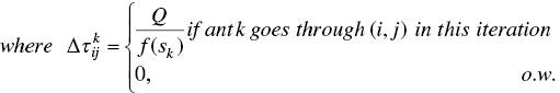
The following equations correspond to the pheromone update strategy of the surgical case sequence problem:
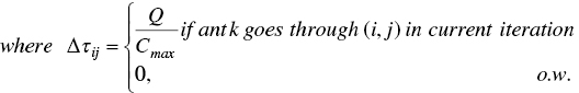
where pheromone evaporation rate is notated by ρ; ∆τij is the incremental pheromone on the edge (i,j), i.e. surgical case i to surgical case j; Q is an adjustable parameter; and Cmax is the makespan of scheduling.

Figure 3.12 Pseudo code of two‐level ACO.
The following equations correspond to the pheromone update strategy for the resource allocation problem as part of the main problem:

where ![]() denotes the pheromone for surgery i with resource m in the selection stage of cth resource type, and
denotes the pheromone for surgery i with resource m in the selection stage of cth resource type, and ![]() is notated for the incremental pheromone on the resource m in the selection stage of cth resource as presented in Eq. (3.26).
is notated for the incremental pheromone on the resource m in the selection stage of cth resource as presented in Eq. (3.26).
The following equation corresponds to the local pheromone update strategy for the resource allocation problem:
where q0 denotes the decremented pheromone value. After updating pheromone locally, the possibility of ants moving through the same path is decreased, and hence the uneven utilization of resources can effectively be avoided.
The transition rule in the outer ant graph (surgery) is presented as the following equation. In the outer surgery graph, the choice probability ![]() of an ant means choosing node (surgical case) j from node (surgical case) i.
of an ant means choosing node (surgical case) j from node (surgical case) i.

Where I0 denotes a feasible solution inclusive of nodes to be scheduled; τij is the outer pheromone value between cases i and j; μij represents the heuristic value from cases i to case j, the two parameters α and β are applied to determine the relative importance of pheromone trail and the heuristic information, respectively. The next case to be chosen is according to the probability, ![]() , where a roulette wheel rule is applied to choose the node.
, where a roulette wheel rule is applied to choose the node.
The transition rule in the inner resource graph is denoted as ![]() , and it presents the probability of choosing resource m for the cth resource type state of surgery i by ant #k:
, and it presents the probability of choosing resource m for the cth resource type state of surgery i by ant #k:

where the inner surgery‐related pheromone is denoted by ![]() and
and ![]() denotes the inner resource‐itself pheromone. The balanced utilization of resources is considered by applying the multiple of these two pheromone values. The parameter in(μcm) is the heuristic information, and G is the available set of resources for selecting the next resource node.
denotes the inner resource‐itself pheromone. The balanced utilization of resources is considered by applying the multiple of these two pheromone values. The parameter in(μcm) is the heuristic information, and G is the available set of resources for selecting the next resource node.
3.3.8 Improved Auto Control ACO with Lazy Ant
In a biological study [18], it was observed that an ant moves from an active state to lazy (inactive) state in some ant colonies. Inspired by this state among ants, an advanced ACO was proposed to solve the grid scheduling problem (GSP) by Tiwari and Vidyarthi [14]. For this purpose, the Auto controlled ACO was developed by incorporating the concept of lazy ants as well as an improved auto‐control mechanism to update parameters. The researchers called their novel method Improved Auto‐Controlled Ant Colony Optimization (IAC‐ACO), in which states of some ants were changed from active to lazy in each iteration. The researchers found that lazy ants ameliorate the intensification strategy, saving computational time.
Lazy ants help the algorithm to speed up convergence of the solution and, moreover, increase the probability of intensification of the solution near the best agent. Therefore, the computational time of the algorithm is reduced by using some lazy ants instead of active ants. To generate lazy ants, a significant portion of its path is copied from the best solution of the current generation. Moreover, at the end of the tour completion, the best ant is separated from the population. To solve the GSP, a few tasks on the different nodes/machine are exchanged. Therefore, the fitter ants in the current iteration are mutated to generate lazy ants. Until the generation of fitter lazy ants in successive iterations, the lazy ants will be alive. This is possible only if lazy ants are empowered with memory.
When the best ant of each generation in a double‐layered structure is saved, the lazy ants are created. The probabilistic decision is not done for constructing the path of a lazy ant; this path is therefore free from the requirements of pheromone values and heuristics. Therefore, in comparison to the active ants, lazy ants consume less time to construct their tour. More than 80% of the route is copied from the best ants of the previous iteration for tour completion, while the rest of the task is mutually swapped among the nodes.
Once the best ant is separated from the population, a few tasks are replaced mutually on some machine, randomly based on the following equation, to generate a set of lazy ants of cardinality h. This process can be done for the k successive best ants. The fitness of lazy ants is computed as was done for the active ants. Thus, the best lazy ants are selected and recorded among the generated k × h lazy ants. The researchers assumed k = 2 and formulated according to the following equation to make the number of ants.

Some novel and diverse researches related to the application of ACO in scheduling problems are displayed in Table 3.2.
Table 3.2 Research related to the application of ACO for scheduling problems.
| Researchers | Approach | Problem |
| [19] | ACO | Scheduling transactions in a grid processing |
| [20] | ACO | Tread scheduling |
| [21] | ACO | Multi‐objective job‐shop scheduling with equal‐size lot‐splitting |
| [22] | ACO | Patient scheduling |
| [23] | ACO | Cyclic job shop robotic cell scheduling problem |
| [24] | ACO | Distributed meta‐scheduling in lambda grids |
| [25] | Graph‐based ACO | Integrated process planning and scheduling |
| [26] | ACO‐DDVO | Irrigation scheduling |
| [27] | ACO | Airline crew scheduling problem |
| [28] | Hybrid ACO | No‐wait flow shop scheduling problems |
| [29] | Modified ACO | Distributed job shop scheduling |
| [30] | Robust ACO | Continuous functions |
| [31] | ACO | Scheduling of agricultural contracting work |
| [32] | Hybrid ACO | Parallel machine scheduling in fuzzy environment |
| [33] | ACO | Multi‐satellite control resource scheduling |
| [34] | Immune ACO | Routing optimization of emergency grain distribution vehicles |
3.4 Introduction to Multi‐Objective Ant Colony Optimization (MOACO)
In this section, we give concise information about the most recent concepts of MOACO, in which non‐dominated solutions are obtained and are used to update global pheromone. These algorithms are just introduced to motivate researchers and practitioners to present new multi‐objective algorithms or extend these algorithms to solve new multi‐objective combinatorial optimization problems.
In the first place, we describe crowding population‐based ant colony optimization (CPACO), introduced by [35] to solve multi‐objective TSP. The researcher extended the traditional algorithm, i.e. population‐based ant colony optimization (PACO) algorithm for solving a problem that applies the super/subpopulation scheme; however, a crowding replacement scheme is applied in the CPACO algorithm. The author emphasizes that this new scheme maintains a preset size of single population (S) and the generated solutions are used to initialize it randomly. A new population of solutions (Y) is created in every generation, and a random subset S′ of S is compared with each new solution to find its closest match. The existing solution is replaced with a new solution if and only if the latter is better than the former solution.
CPACO applies different heuristic matrices with the same pheromone trail for each objective and initializes the pheromone matrix with some initial value τinit. After that, the pheromone values of all solutions are updated in each generation according to their inverse of the rank as follows:

The dominance ranking method is applied to assign an integer rank for all solutions in the population. The notation of λ denotes a correction factor that is related to the heuristic information, and it is generated by CPACO for each objective function (d). Therefore, each ant can utilize a different amount of heuristic based on this factor. Transition rule probability is calculated using the following equation:

The measures that are applied to test the performance of the CPACO algorithm include dominance ranking and attainment surface comparison. To evaluate the closeness of solutions to the Pareto front and to increase the diversity of solutions, the measures above are applied. Furthermore, statistical analysis indicates that the CPACO algorithm outperforms the traditional method. The CPACO algorithm records a smaller population than the traditional algorithm. CPACO uses the sorting method and PACO applies the average‐rank‐weight method to rank the objectives. Consequently, the computational complexity of CPACO is lower than that of PACO.
In the next place, we present Pareto strength ant colony optimization (PSACO), which was proposed by [36] to solve the multi‐objective problem. This algorithm is based on the first ant colony groups; AS and the domination concept of the strength Pareto evolutionary algorithm (SPEA‐II) introduced by [37] are applied for optimizing the multi‐objective TSP problem. This algorithm makes two sets of solutions; population Pt and archive At for each iteration t. Solutions generated by the current iteration are maintained in the set of Pt and, moreover, a fixed number of globally best non‐dominated solutions are saved in the archive set. If the size of the archive exceeds the fixed value, it is truncated by the current best dominant solutions. S(i) in Eq. (3.33) is a strength value that shows the number of the solutions dominated in the population and archive by each individual.
where the cardinality of a set is denoted by |.| and i > j represents that solution i dominates solution j. To evaluate the quality of each solution Q(i) as formulated in Eq. (3.33), two other partial values are calculated. The fitness of each individual is based on S(i) and is represented by R(i). Furthermore, D(i) shows the density information of each individual that is computed by using the kth nearest neighbor (KNN) method.

The pheromone update procedure of this algorithm is formulated as Eqs. (3.34) and (3.35):

where Q(k) is the solution cost of kth ant according to the Q(i) calculation.
3.5 Keywords Analysis for Application of ACO in Scheduling
After a brief review of ACO history, the scientometric analysis was applied using the keywords “Ant colony optimization” and “Scheduling.” To this end, the titles “Ant colony optimization” and “Scheduling” were searched in SCOPUS database, which returned approximately 1746 scientific articles between 1970 and early 2018. The search was done among keywords in “article title,” “author keywords,” and “abstract.” Figure 3.13 shows a cognitive map where the number of documents is equal to the size of the node on the mentioned term, and links among disciplines are presented by a line, and its density is relative to the level of which two areas were being used in one paper. Shadings are used to show the cluster of each item to which it belongs.
The significant keywords (five most significant and five least significant keywords) and their number of occurrences have been presented in Table 3.3. The goal of this analysis (keyword search) is to analyze the terms as regards accuracy. This analysis mainly uses brainstorming to find the crucial keywords that still have a high or low number of searches.

Figure 3.13 Cognitive map (co‐occurrences for keyword search).
Table 3.3 The significant keywords in the application of ACO in scheduling.
| No. | Keyword | Occurrences |
| 1 | Scheduling | 915 |
| 2 | Ant colony optimization | 897 |
| 3 | Optimization | 810 |
| 4 | algorithms | 625 |
| 5 | Artificial intelligence | 562 |
| 6 | Surgery scheduling | 6 |
| 7 | Hospital management | 4 |
| 8 | Human | 4 |
| 9 | Working time | 5 |
| 10 | Cellular manufacturing | 8 |
3.6 Application of Bi‐Objective Ant Colony Optimization in Healthcare Scheduling
3.6.1 Problem Statement
In this section, we give a brief description of surgical case processing from input to output in operating theaters (Figure 3.14). Firstly, the patient is transported from either the ward as an inpatient or ASU as an outpatient to PHU. While the patient is being held in PHU, the nurse checks their documents and prepares him/her for surgery.
The patient occupies both a nurse and a PHU bed. Then he/she is moved to an operating room where an anesthetist manages the anesthesia process, and a specific surgeon performs a surgical procedure on the case. During this stage, other resources such as a nurse, OR, anesthetist, medical technicians, scrubs, and surgeon are allocated to the surgical case. At the end of the surgical process, anesthesia is reversed by anesthetist, and then the patient is transported to PACU, where he/she recovers from the residual effects of anesthesia under the care of a PACU nurse. For the third stage, a nurse and a PACU bed are assigned to the patient.
In addition to patient flow in Figure 3.14, the sequence of the surgical case is presented. As shown, surgical cases (SC1 ,…,SCj) are sequenced and, moreover, efficient available resources are allocated to them in order to minimize makespan (Cmax) and minimize the number of the non‐scheduled surgical cases within the interval between the end of the time window (EW) and the start of the time window (SW). Also, multi‐resources assigned to the jth surgical case for each stage are presented by blue boxes over the SCj .
The various structures of the shop are taken into account to model and solve the SCS problem. For instance, [38] formulated a two‐stage hybrid flow shop model in order to minimize total overtime in operating rooms, and [39] modeled the SCS problem as a four‐stage flow shop under open scheduling policy. In other studies [13, 40, 41], the similarities between the operating room scheduling environment and job shop scheduling were observed. An FJS is introduced by Pinedo [42] as a generalization of the job shop with the incorporation of the parallel machine environments. Each order has its route to follow through the shop. Even though the flow shop may be modeled for an operating theater in the case of identical surgical procedures, in the real world each surgical case is processed by a special surgeon and therefore the job shop environment is suitable for this problem. Pham and Klinkert [40] developed novel multi‐mode blocking job shop scheduling to model the SCS problem in order to minimize makespan. However, [13] considered the generalization of the job shop and then formulated a multi‐resource FJSP in order to minimize makespan. They assumed that the operating sequence of three stages must be followed completely and in sequence, so this assumption makes a constraint that follows the rules of a no‐wait flow shop.

Figure 3.14 Patient processing in operating theater and surgical case scheduling in operating theater.
Pinedo defined the no‐wait requirement as a phenomenon that may occur in flow shops with zero intermediate storage. In the no‐wait situation, orders are not permitted to wait between two successive machines. By using this constraint in FJSP, the starting time of the first stage in PHU for the surgical case has to be delayed to ensure that the case can go through the FJS without having to wait for any resource. Therefore, the surgical cases are pulled down the line by resources that have become idle. On the other hand, [13] assumed that three general stages are essential for all cases in FJS. We can observe flexibility in all stages because of the diversification in resources of each stage.
3.6.2 Introduction to Pareto Enveloped Selection Ant System (PESAS)
In this section, we suggest metaheuristic approaches in order to tackle the combinatorial nature of the bi‐objective surgical case scheduling (BOSCS) problem. In many studies in the field of operating room scheduling problems, some heuristic or metaheuristic procedures such as NSGA‐II from genetic algorithm family [43, 44], tabu search [45, 46], column generation based heuristic [47], Monte‐Carlo along with genetic algorithm [41], and ACO [13, 48] were developed to achieve near‐optimal solutions.
As noted, [13] proposed an ACO algorithm with a two‐level hierarchical graph (outer and inner graph) to solve SCS. They took into account outer and inner graphs in order to integrate sequencing surgical cases and to allocate resources simultaneously. Therefore, we extend a two‐level ACO algorithm to a bi‐objective two‐level ACO for solving the optimization problem. To the best of our knowledge, in the area of BOSCS in literature, no research is available that employs any versions of the multi‐objective ACO algorithm. Therefore, we apply pheromone updating of MMAS along with non‐dominated concepts of a Pareto envelope‐based selection algorithm (PESA‐II) in order to construct a new algorithm from multi‐objective ACO groups for solving the problem. Then we compare our proposed solution procedure with Pareto strength ant colony optimization (PSACO), which was articulated in the fourth section, and hence the efficiency of the method is determined according to the several metrics of multi‐objective algorithms. The traditional algorithm is based on the proposed MOACO by [36], and our proposed algorithm called Pareto envelope‐based selection ant system (PESAS), which was developed by applying rules of PESA‐II along with the pheromone updating strategy of the Xiang algorithm. Therefore, we contribute to new knowledge with the extension of Xiang's model so that we develop a single objective ACO algorithm to the bi‐objective algorithm. In the proposed algorithm, two‐level ACO is extended to the bi‐objective ant colony optimization approach by using the rules of pheromone update strategy of MMAS along with the domination concept of PESA‐II [49].
In the PESAS algorithm, two agent sets include the population of ants (Antt) and the repository (Rept) is made in each iteration. Solutions produced by the current iteration are recorded in the set of Antt and then a fixed number of globally non‐dominated solutions are saved in repository set, and this fixed number is based on a threshold of the repository (Repth ). In the current iteration, the solutions of the repository are updated by generated non‐dominated agents. Since an agent solution from the repository must be selected for pheromone updating, a grid is created according to the evolutionary concepts in PESA‐II that solution selecting is region‐based not individual‐based. In region‐based selection, each cell space of the grid with less population is more probable to be selected to improve the diversity of the algorithm. After creation of grid, it is rechecked that the number of repository solutions must be less than Repth ; otherwise, the excessive population of the repository is eliminated according to the selection probability of cell space that cells with more population are more probable for selection. For example, as indicated in Figure 3.15, light gray (near the numbers) are non‐dominated solutions of the repository and dark gray (further to the right) show dominated ant populations. For example, cells #1 and #3 are selected with more probability for updating pheromone, and the population of cell #2 is more likely to be eliminated if the total number in the repository exceeds the threshold.
The selection probability rule of the cells for pheromone updating is based on Roulette Wheel Selection (RWS) and is formulated as follows:

where β is the selection pressure of the cell for pheromone updating, n denotes the number of the cells in repository space, ni is the population of ith cell, and Pi is the probability selection of ith cell. It should be noted that if the population of the selected cell is more than 1, one is selected randomly according to a uniform distribution.

Figure 3.15 Sample of bi‐objective space of ant solutions (f1, f2) with grid.
Besides, the selection probability rule of the cells for eliminating is based on RWS and is formulated as follows:

where γ is the selection pressure of the cell for eliminating, n denotes the number of cells in repository space, ni is a population of ith cell, and qi is the probability selection of ith cell. It must be noted that if the population of the selected cell is more than 1, one is selected randomly according to a uniform distribution.
To update the trail pheromone, we follow the updating equations of MMAS proposed by [9]:

and pheromone deposited based on a selected non‐dominated solution by using region‐based selection (nd). Also, S(i) is called strength value and indicates the number of the solutions dominated in current population and repository by each, as used in the PSACO. In this approach, the ant is selected according to Eq. (3.30) for updating.
3.6.3 Results and Discussion
3.6.3.1 Illustrative Examples
To evaluate the proposed approaches, we took three test surgery cases. These cases are classified into small, medium, and large, which differed as regards surgery duration, the number of the surgery cases, and the allocated resources. Case categories and their specifications are shown in Table 3.4. As can be seen, the three problems of each case are different in size of surgeries (column 3), size of resources (column 4–9), and surgery type structure (column 10). The algorithms were coded in Matlab language and ran on an Intel Core (TM) Duo CPU T2450, 2.00 GHz computer with 1 GB of RAM.
3.6.3.2 Performance Evaluation Metrics
In this section, some main performance metrics are applied in order to evaluate the quality and diversity of the obtained non‐dominated solutions in the Pareto repository set of the PESAS algorithm. There are three critical metrics in the literature of multiple objective problems [50], which we describe as follows:
Table 3.4 Test cases and structure.
| Cases | Problem | Surgical case | PHU bed | Nurse | Surgeons | ORs | PACU bed | Anesthesia | Surgery type (S:M:L:EL:S) |
| Case1 | 1 | 8 | 1 | 5 | 5 | 2 | 2 | 5 | 2:4:1:1:0 2:6:1:1:0 |
| 2 | 10 | 2 | 8 | 6 | 4 | 4 | 6 | ||
| 3 | 10 | 2 | 8 | 6 | 4 | 4 | 6 | 2:5:2:1:0 | |
| Case2 | 1 | 15 | 3 | 10 | 6 | 4 | 3 | 8 | 3:9:2:1:0 |
| 2 | 20 | 3 | 15 | 10 | 5 | 4 | 8 | 4:12:3:1:0 | |
| 3 | 20 | 3 | 15 | 10 | 5 | 4 | 8 | 4:10:3:3:0 | |
| Case3 | 1 | 30 | 4 | 19 | 10 | 6 | 5 | 9 | 7:16:3:2:2 |
| 2 | 30 | 4 | 22 | 12 | 6 | 5 | 11 | 5:15:3:4:3 | |
| 3 | 30 | 5 | 22 | 12 | 6 | 6 | 12 | 3:15:3:4:5 |
- Quality metric ( QM ). This metric was proposed by [51] and takes into account the number of Pareto solutions obtained by each algorithm. In other words, non‐dominated solutions of all algorithms are compared and then the algorithm with a higher number of final Pareto solutions has more quality. It is clear that the larger the QM, the better the obtained solution set.
(3.41)

where, ![]() denotes the final Pareto solution set of both algorithms and N is the number of the final obtained Pareto solutions that contains Np1 and Np2 .
denotes the final Pareto solution set of both algorithms and N is the number of the final obtained Pareto solutions that contains Np1 and Np2 .
- Spacing metric ( SM ).This metric was employed by [52] in order to assess the uniformity of the spread of the solutions in the final Pareto solution set obtained by each algorithm, and it is computed as follows:
(3.42)
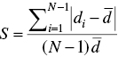
where, di denotes the Euclidean distance between the two solutions of the Pareto set, ![]() denotes the average value of all Euclidean distances, and N is the number of final Pareto solutions found. It is obvious that the smaller the SM, the better spacing of the Pareto set and the best value for this metric is equal to 0.
denotes the average value of all Euclidean distances, and N is the number of final Pareto solutions found. It is obvious that the smaller the SM, the better spacing of the Pareto set and the best value for this metric is equal to 0.
- Diversity metric ( DM ). This metric was used by [53] and was employed to evaluate the spread of the solutions in the final Pareto set of each algorithm. This metric is formulated as follows:
(3.43)
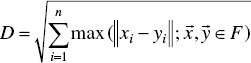
where F denotes the set of found Pareto, ![]() and
and ![]() denotes two solution vectors of Pareto frontier, and n represents the dimension of the solution space or, in other words, the number of the objective functions. It is clear that the larger the DM, the better the generated Pareto set.
denotes two solution vectors of Pareto frontier, and n represents the dimension of the solution space or, in other words, the number of the objective functions. It is clear that the larger the DM, the better the generated Pareto set.
3.6.3.3 Comparison between the Algorithm's Performance on all Considered Instances
The proposed algorithm was run 10 times for each instance tested in order to compare with other traditional algorithms.
Table 3.5 indicates the average performance of our proposed algorithm and comparison to PSACO as an important method for solving all instances. The first and second columns display considered test problems and approaches, respectively. The next three columns represent the average, best, and worst of the QM for solutions obtained. The average, best, and worst of the diversity metric for solutions are given from the sixth to eighth columns of the table. Also, the following three columns present the results of SM. [54] introduced a two‐time index to compare the computational time of algorithms, namely A1 (s) the average computational times for obtaining one solution and A2 (s) the average computational times for all solutions found. The last two columns of the table give results of A1 (s) and A2 (s) after 10 runs. These computational time criteria are formulated as follows:


Where ![]() denotes the number of the solutions found in the ith run, ti represents the computational times for the ith run, and w is running time.
denotes the number of the solutions found in the ith run, ti represents the computational times for the ith run, and w is running time.
As the table shows, PESAS outperforms PSACO for solving all instances from small to large size in three metrics (quality, diversity, and spacing), with the exception of the diversity metric for instance #1 and the best SM obtained for instances #6 and #9, where PSACO yields better metrics. Nevertheless, the optimal non‐dominated solutions found by PESAS are better than those of PSACO for all test cases. Since our proposed algorithm uses only a diverse dominant agent to update the pheromone trail, it seems that the results of PESAS outperform the results of PSACO, which uses all dominant ants to update the pheromone. It seems that having diverse dominant ants increases the diversification strategy of the algorithm to find a better Pareto front, and the results indicate this assumption. On the other hand, the average of the computational time (A2) of PSACO is less than that of PESAS, and the reasons for this extra time relate to the existence of the grid‐based selection procedure in our proposed algorithm. However, our proposed algorithm requires less effort for finding an optimal solution in comparison with PSACO based on A1 (s) measurement.
Table 3.5 Comparison of the performance of the algorithms on all considered test case problems.
| Problems | Algorithms | QM | DM | SM | A1(s)a | A2(s)a | Average | Best | Worst | Average | Best | Worst | Average | Best | Worst |
| Instance1 | PESAS | 3.9 | 5 | 3 | 139.066 | 156 | 128.03 | 0.7228 | 0.268 | 0.99 | 4.9443 | 19.283 | |||
| PSACO | 0.1 | 1 | 0 | 145.814 | 163.05 | 120.04 | 1.059 | 0.55 | 1.68 | 186.87 | 18.687 | ||||
| Instance2 | PESAS | 6.4 | 7 | 5 | 167.404 | 179.1 | 159.1 | 0.568 | 0.4 | 0.8 | 4.1542 | 26.587 | |||
| PSACO | 0.3 | 1 | 0 | 141.613 | 159.11 | 132 | 0.993 | 0.46 | 1.43 | 89.34 | 26.802 | ||||
| Instance3 | PESAS | 7.8 | 9 | 7 | 182.619 | 191.16 | 170.14 | 0.631 | 0.47 | 0.8 | 3.3124 | 25.837 | |||
| PSACO | 0.1 | 1 | 0 | 167.535 | 188.2 | 122.14 | 0.831 | 0.58 | 1.16 | 265.5 | 26.55 | ||||
| Instance4 | PESAS | 9.5 | 10 | 8 | 177.79 | 196.2 | 162.25 | 0.497 | 0.29 | 0.76 | 3.9363 | 37.395 | |||
| PSACO | 0 | 0 | 0 | 172.48 | 196.16 | 155.16 | 0.846 | 0.43 | 1.12 | infinite | 31.218 | ||||
| Instance5 | PESAS | 11.4 | 12 | 10 | 189.777 | 206.4 | 171 | 0.466 | 0.34 | 0.59 | 7.9447 | 90.57 | |||
| PSACO | 0.5 | 1 | 0 | 184.47 | 205 | 167.3 | 0.787 | 0.5 | 1.12 | 158.34 | 79.17 | ||||
| Instance6 | PESAS | 7.8 | 9 | 5 | 185.9873 | 212.8 | 169.9 | 0.4239 | 0.12 | 0.7 | 13.871 | 108.2 | |||
| PSACO | 0.6 | 3 | 0 | 165.67 | 188 | 144.3 | 0.636 | 0.42 | 1.09 | 161.583 | 96.95 | ||||
| Instance7 | PESAS | 11.5 | 17 | 8 | 290.404 | 307.59 | 254.33 | 0.5019 | 0.29 | 0.67 | 17.0143 | 195.665 | |||
| PSACO | 1.6 | 7 | 0 | 259.611 | 291.4 | 220.5 | 0.675 | 0.48 | 0.89 | 116.461 | 186.339 | ||||
| Instance8 | PESAS | 9.3 | 13 | 3 | 324.888 | 344.37 | 290.5 | 0.577 | 0.34 | 0.82 | 21.5433 | 200.353 | |||
| PSACO | 2.9 | 7 | 0 | 289.327 | 345 | 246.4 | 0.663 | 0.37 | 0.91 | 64.8520 | 188.071 | ||||
| Instance9 | PESAS | 7.1 | 14 | 3 | 320.423 | 376.6 | 299.6 | 0.528 | 0.32 | 0.82 | 29.7419 | 211.168 | |||
| PSACO | 2.9 | 7 | 0 | 302.033 | 355 | 263.4 | 0.523 | 0.22 | 0.9 | 72.8351 | 211.222 |
a Time unit: second.
Figure 3.16 Interaction between the algorithms and test samples for the quality measure.
Figure 3.17 Interaction between the algorithms and test samples for the diversity measure.

Figure 3.18 Interaction between the algorithms and test samples for the spacing measure.
Figure 3.16 shows that the proposed PESAS algorithm obtains more Pareto solutions than the other algorithm for each instance and therefore our method outperforms PSACO. Figure 3.17 indicates that the proposed PESAS algorithm obtains more diverse solutions than the other algorithm for each instance except instance 1. Thus our method outperforms PSACO. Figure 3.18 indicates that the proposed PESAS algorithm obtains solutions with less space metric than another algorithm for each instance except instance #6 and #9 in best SM obtained. Therefore, our method outperforms PSACO.
References
- 1 Dorigo, M., Maniezzo, V., and Colorni, A. (1991). Positive feedback as a search strategy (Tech. Rep. No. 91‐016). Politecnico di Milano, Milan, Italy.
- 2 Dorigo, M. and Gambardella, L.M. (1997). Ant colony system: a cooperative learning approach to the traveling salesman problem. IEEE Trans. Evol. Comput. 1: 53–66.
- 3 Deneubourg, J.‐L., Aron, S., Goss, S., and Pasteels, J.M. (1990). The self‐organizing exploratory pattern of the argentine ant. J. Insect Behav. 3: 159–168.
- 4 Blum, C. and Roli, A. (2003). Metaheuristics in combinatorial optimization: overview and conceptual comparison. ACM Comput. Surveys (CSUR) 35: 268–308.
- 5 Dorigo, M. and Blum, C. (2005). Ant colony optimization theory: a survey. Theor. Comput. Sci. 344: 243–278.
- 6 Yang, X.‐S. (2010). Nature‐Inspired Metaheuristic Algorithms. Luniver Press.
- 7Dorigo, M. (1992). Optimization, learning and natural algorithms. PhD thesis. Politecnico di Milano.
- 8 Bullnheimer, B., Hartl, R.F., and Strauss, C. (1997). A new rank based version of the Ant System. A computational study. Centr. Eur. J Operat. Res. 7: 25–38.
- 9 Stützle, T. and Hoos, H.H. (2000). MAX–MIN ant system. Future Gener. Comput. Syst. 16: 889–914.
- 10 Cordon, O., de Viana, I.F., Herrera, F., and Moreno, L. (2000). A new ACO model integrating evolutionary computation concepts: The best‐worst Ant System. Proc Ants'2000. 22–29.
- 11 Guntsch, M. and Middendorf, M. (2002b). A population based approach for ACO. Workshops on Applications of Evolutionary Computation 72–81. Springer.
- 12 Blum, C. (2005). Beam‐ACO—hybridizing ant colony optimization with beam search: an application to open shop scheduling. Comput. Oper. Res. 32: 1565–1591.
- 13 Xiang, W., Yin, J., and Lim, G. (2015). An ant colony optimization approach for solving an operating room surgery scheduling problem. Comput. Ind. Eng. 85: 335–345.
- 14 Tiwari, P.K. and Vidyarthi, D.P. (2016). Improved auto control ant colony optimization using lazy ant approach for grid scheduling problem. Future Gener. Comput. Syst. 60: 78–89.
- 15 Cordón, O., de Viana, I.F., and Herrera, F. (2002). Analysis of the best‐worst ant system and its variants on the QAP. International Workshop on Ant Algorithms, 228–234. Springer.
- 16 Guntsch, M. and Middendorf, M. (2002). Applying population based ACO to dynamic optimization problems. International Workshop on Ant Algorithms, 111–122. Springer.
- 17 Ow, P.S. and Morton, T.E. (1988). Filtered beam search in scheduling. Int. J. Prod. Res. 26: 35–62.
- 18 Gordon, D.M., Goodwin, B.C., and Trainor, L.E.H. (1992). A parallel distributed model of the behavior of ant colonies. Theoret. Biol. 156 (3): 293–307.
- 19 Mahato, D.P., Singh, R.S., Tripathi, A.K., and Maurya, A.K. (2017). On scheduling transactions in a grid processing system considering load through ant colony optimization. Appl. Soft Comput. 61: 875–891.
- 20 Anjaria, K. and Mishra, A. (2017). Thread scheduling using ant colony optimization: an intelligent scheduling approach towards minimal information leakage. Karbala Int. J. Modern Sci. 3: 241–258.
- 21 Huang, R.‐H. and Yu, T.‐H. (2017). An effective ant colony optimization algorithm for multi‐objective job‐shop scheduling with equal‐size lot‐splitting. Appl. Soft Comput. 57: 642–656.
- 22 Obiniyi, A. (2015). Multi‐agent based patient scheduling using ant colony optimization. Afr. J. Comput. ICT 8: 91–96.
- 23Elmi, A. and Topaloglu, S. (2017). Cyclic job shop robotic cell scheduling problem: ant colony optimization. Comput. Ind. Eng. 111: 417–432.
- 24 Pavani, G.S. and Tinini, R.I. (2016). Distributed meta‐scheduling in lambda grids by means of ant colony optimization. Future Gener. Comput. Syst. 63: 15–24.
- 25 Wang, J., Fan, X., Zhang, C., and Wan, S. (2014). A graph‐based ant colony optimization approach for integrated process planning and scheduling. Chin. J. Chem. Eng. 22: 748–753.
- 26 Nguyen, D.C.H., Ascough, J.C. II, Maier, H.R. et al. (2017). Optimization of irrigation scheduling using ant colony algorithms and an advanced cropping system model. Environ. Model. Software 97: 32–45.
- 27 Deng, G.‐F. and Lin, W.‐T. (2011). Ant colony optimization‐based algorithm for airline crew scheduling problem. Expert Syst. Appl. 38: 5787–5793.
- 28 Engin, O. and Güçlü, A. (2018). A new hybrid ant colony optimization algorithm for solving the no‐wait flow shop scheduling problems. Appl. Soft Comput. 72: 166–176.
- 29 Chaouch, I., Driss, O.B., and Ghedira, K. (2017). A modified ant colony optimization algorithm for the distributed job shop scheduling problem. Procedia Comput. Sci. 112: 296–305.
- 30 Chen, Z., Zhou, S., and Luo, J. (2017). A robust ant colony optimization for continuous functions. Expert Syst. Appl. 81: 309–320.
- 31 Alaiso, S., Backman, J., and Visala, A. (2013). Ant colony optimization for scheduling of agricultural contracting work. IFAC Proc. Vol. 46: 133–137.
- 32 Liao, T.W. and Su, P. (2017). Parallel machine scheduling in fuzzy environment with hybrid ant colony optimization including a comparison of fuzzy number ranking methods in consideration of spread of fuzziness. Appl. Soft Comput. 56: 65–81.
- 33 Zhang, Z., Zhang, N., and Feng, Z. (2014). Multi‐satellite control resource scheduling based on ant colony optimization. Expert Syst. Appl. 41: 2816–2823.
- 34 Zhang, Q. and Xiong, S. (2018). Routing optimization of emergency grain distribution vehicles using the immune ant colony optimization algorithm. Appl. Soft Comput. 71: 917–925.
- 35 Angus, D. (2007). Crowding population‐based ant colony optimisation for the multi‐objective travelling salesman problem. IEEE Symposium on Computational Intelligence in Multicriteria Decision Making, 333–340.
- 36 Thantulage, G.I. (2009). Ant colony optimization based simulation of 3D automatic hose/pipe routing. PhD thesis. Brunel University School of Engineering and Design.
- 37 Zitzler, E., Laumanns, M., and Thiele, L. (2001). SPEA2: Improving the Strength Pareto Evolutionary Algorithm. TIK‐report 103.
- 38 Guinet, A. and Chaabane, S. (2003). Operating theatre planning. Int J. Prod. Econ. 85: 69–81.
- 39Augusto, V., Xie, X., and Perdomo, V. (2010). Operating theatre scheduling with patient recovery in both operating rooms and recovery beds. Comput. Ind. Eng. 58: 231–238.
- 40 Pham, D.‐N. and Klinkert, A. (2008). Surgical case scheduling as a generalized job shop scheduling problem. Eur. J. Oper. Res. 185: 1011–1025.
- 41 Lee, S. and Yih, Y. (2014). Reducing patient‐flow delays in surgical suites through determining start‐times of surgical cases. Eur. J. Oper. Res. 238: 620–629.
- 42 Pinedo, M.L. (2008). Scheduling: Theory, Algorithms, and Systems. New York: Springer.
- 43 Marques, I. and Captivo, M.E. (2015). Bicriteria elective surgery scheduling using an evolutionary algorithm. Oper. Res. Health Care 7: 14–26.
- 44 Marques, I., Captivo, M.E., and Pato, M.V. (2014). Scheduling elective surgeries in a Portuguese hospital using a genetic heuristic. Oper. Res. Health Care 3: 59–72.
- 45 Lamiri, M., Grimaud, F., and Xie, X. (2009). Optimization methods for a stochastic surgery planning problem. Int J. Prod. Econ. 120: 400–410.
- 46 Saremi, A., Jula, P., Elmekkawy, T., and Wang, G.G. (2013). Appointment scheduling of outpatient surgical services in a multistage operating room department. Int J. Prod. Econ. 141: 646–658.
- 47 Fei, H., Meskens, N., and Chu, C. (2010). A planning and scheduling problem for an operating theatre using an open scheduling strategy. Comput. Ind. Eng. 58: 221–230.
- 48 Behmanesh, R., Zandieh, M., and Hadji Molana, S.M. (2019). The surgical case scheduling problem with fuzzy duration time: an ant system algorithm. Sci. Iran. 26 (3): 1824–1841.
- 49 Corne, D.W., Jerram, N.R., Knowles, J.D., and Oates, M.J. (2001). PESA‐II: region‐based selection in evolutionary multiobjective optimization. Proceedings of the 3rd Annual Conference on Genetic and Evolutionary Computation, 283–290. Morgan Kaufmann Publishers Inc.
- 50 Noori‐Darvish, S., Mahdavi, I., and Mahdavi‐Amiri, N. (2012). A bi‐objective possibilistic programming model for open shop scheduling problems with sequence‐dependent setup times, fuzzy processing times, and fuzzy due dates. Appl. Soft Comput. 12: 1399–1416.
- 51 Schaffer, J.D. (1985). Multiple objective optimization with vector evaluated genetic algorithms. Proceedings of the First International Conference on Genetic Algorithms and Their Applications, Lawrence Erlbaum Associates. Inc., Publishers.
- 52 Svinivas, N. (1995). Multiobjective optimization using nondominated sorting in genetic algorithms. IEEE Trans. Evol. Comput. 2: 221–248.
- 53 Zitzler, E. (1999). Evolutionary Algorithms for Multiobjective Optimization: Methods and Applications. Citeseer.
- 54 Li, J.‐Q., Pan, Q.‐K., and Tasgetiren, M.F. (2014). A discrete artificial bee colony algorithm for the multi‐objective flexible job‐shop scheduling problem with maintenance activities. App. Math. Model. 38: 1111–1132.