CHAPTER 1
Theory
In this chapter, we will introduce some basic concepts of equity modeling. We will discuss how the stock price can be modeled in a framework with deterministic interest rates, dividends, and default probabilities and how a given implied volatility surface can be matched with Dupire's “implied local volatility.” We also mention alternatives and how European payoffs whose value depends only on the stock price on a single maturity can be priced independent of further model assumptions by hedging with European options. We also make a few remarks on theoretical aspects of replication. This chapter is the foundation of chapter 2, where we will discuss applications: various stochastic volatility models, pricing of Cliquets, variance swaps, and related products and models to price options on variance. The assumptions of deterministic interest rates and default risk probabilities are then subsequently relaxed in the later chapters of this book.
1.1 CONCEPTS OF EQUITY MODELING
Since the main focus of this chapter is the modeling of the pure equity risk, we will work with a framework where interest rates, dividends, and default risk are deterministic. We will model the stock price on a stochastic base ![]()
![]() The measure
The measure ![]() is the “historic” measure. We denote by r = (rt)t≥0 the deterministic interest rates and we use μ = (μt)t≥0 to refer to a deterministic repo rate (it represents the gains we make from lending out a share). We will also use B for the cash bond (or “money market account”), that is,
is the “historic” measure. We denote by r = (rt)t≥0 the deterministic interest rates and we use μ = (μt)t≥0 to refer to a deterministic repo rate (it represents the gains we make from lending out a share). We will also use B for the cash bond (or “money market account”), that is,
![]()
and
![]()
for the price at time t of a zero bond with maturity T (see chapter 3 for the case of stochastic interest rates). We also assume that the stock can default: In the event of default, whose time we denote by τ, we stipulate that the value of the share drops to zero. We also assume that corporate zero bonds of the company we want to model are traded for all maturities, and that the value of any outstanding bonds will also drop to zero in the event of default (in practice, this rarely happens: usually, a bond will have some “recovery value,” which represents the fraction of the notional that the defaulted company is still able to pay).1 Since the “risky” corporate zero bond can default, its price at any time prior to τ must be less than the price of the “riskless” government zero bond with same maturity and notional: the zero bond is trading at a spread. We will assume that this spread, or hazard rate, h = (ht)t≥0, of the risky bond interest rate over the riskless rate r, is deterministic, such that the price of the risky zero bond with maturity T at time t is given as
![]()
(Our restriction to deterministic hazard rates will be lifted in chapter 6, where we discuss approaches to model h as a stochastic process.) The default event τ itself is then modeled as an inaccessible exponentially distributed stopping time with intensity h, which is assumed to be independent from the filtration ![]() (i.e., of stock price, interest rates, volatility, etc.).2 Inaccessibility means that the default cannot be foretold by observations of the stock price: It excludes, for example, stopping times that are the result of the stock price crossing some barrier.3 In this setting, we assume, under any pricing measure
(i.e., of stock price, interest rates, volatility, etc.).2 Inaccessibility means that the default cannot be foretold by observations of the stock price: It excludes, for example, stopping times that are the result of the stock price crossing some barrier.3 In this setting, we assume, under any pricing measure ![]() equivalent to
equivalent to ![]() that
that
which implies the intuitive relation ![]() (i.e., the price of the risky bond is the price of the riskless bond times the probability of default). Moreover, our assumptions that zero bonds are available for all maturities, implies that we can roll over a capital investment of 1 into the risky zero bonds and thereby generate a risky cash bond,
(i.e., the price of the risky bond is the price of the riskless bond times the probability of default). Moreover, our assumptions that zero bonds are available for all maturities, implies that we can roll over a capital investment of 1 into the risky zero bonds and thereby generate a risky cash bond,
![]()
which will also drop to zero in the event of default.
As mentioned above, the availability of both the risky and the riskless bond allows us to synthesize a payoff of 1 if the company has defaulted up to some maturity T. As a consequence, we can hedge out the risk of default when pricing an option. A put written on the stock S = (St)t≥0, for example, can be decomposed into
![]()
Hence, we can split its value in the “default value” K1τ≤T, which we can hedge by entering into a long position in a risky zero bond and a short position in a riskless zero bond, and the “survival value” (K − ST)+1τ>T, whose hedge we can approach using standard replication theory, as explained in section 1.4.
1.1.1 The Forward
We also assume that the stock pays dividends. On each of the dividend dates 0 =: τ0 < τ1 < τ2 …, we assume that first a proportional dividend of βk = 1 − e−dk and then a cash dividend of αk is paid. As a result, the stock price at a dividend date will drop by the relative amount e−dk = 1 − βk and the absolute amount αk. Of course, dividends are only paid if the stock did not yet default. Hence, if we assume that the stock price process S = (St)t≥0 only jumps due to dividends, at each dividend date τk < τ, we have
In this setting, let us derive the value of a forward contract with delivery time T: Assume first we buy η shares today and that we short ηS0 riskless zero bonds in order to borrow the required initial capital.4 Since we hold the stock we will earn repo and receive the dividends it pays. To handle them, we decide to reinvest all proportional dividends and proceeds from repo contracts into the stock. Since we receive as many cash dividends as we hold units of stock, this implies that at any time τk before default, we receive an amount of
![]()
We will use these proceedings to buy back our initially issued debt. If the stock does not default, this implies that at time T, we hold
![]()
units of stock and that we are short

units of the zero bond. In order to be able to deliver exactly one share in time T, we chose ![]() such that our terminal capital reads
such that our terminal capital reads

which is therefore the fair strike conditional on no default. However, if there is a default at some time 0 < τ < T, then we will forgo the dividends thereafter. Hence, if we receive K for the share at T, we will be short the missing dividend amounts.
To protect ourselves against default, we need a mechanism which ensures that our terminal bank account always has the same value at time T, be there default or not. This can be achieved if we “forward-sell” the proceeds of the dividends. To this end, we sell “risky” (corporate) zero bonds with maturities 0 < τ1 < … < τN (where τN ≤ T < τN+1). Each bond has a notional of
![]()
and since we hold the appropriate amount of shares at any time before default, we will always be able to fulfill our obligations arising from shorting the bonds. However, since the bond is risky, we have to pay a risk premium of h to the buyers of these bonds, so shorting the bonds yields only
![]()
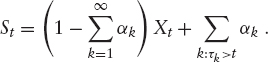
Summing up, we find that the forward strike on S with maturity T is given as

Hence, in the absence of cash dividends, the fair forward strike for an asset does not depend on the default risk involved. Note that F must in all cases be non-negative due to no-arbitrage constraints.
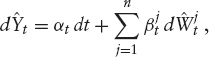
1.1.2 The Shape of Dividends to Come
Given the form of the forward (1.3), what are the implications for potential stock price processes? Between the discrete cash dividends, standard no-arbitrage arguments show that if there is “no free lunch with vanishing risk,”5 then there exists a measure ![]() , equivalent to
, equivalent to ![]() , and a local
, and a local ![]() -martingale Y such that
-martingale Y such that
![]()
holds for t ∈ [τk−1, τk). In τk, equation (1.2) applies and we get, added up,

However, Y is also subject to the constraint that the process S cannot become negative. We will now investigate the impact of this property. The following
discussion holds for local martingales in general, but we focus on the relevant true martingale case. For ease of exposure, let us briefly assume that S0 = 1, r ≡ 0, μ ≡ 0, h ≡ 0 and di ≡ 0, that is, with θ/θ = θ,

At any point t, the forward of the stock to a later date T > t must remain non-negative. This implies that at any dividend date τk, the stock price must exceed the value of all forthcoming dividends,

Since a martingale M with unit mean that is bounded from below by some ![]() ∈ [0, 1] can be written as
∈ [0, 1] can be written as ![]() in terms of a non-negative martingale M+ which has again unit mean, we can write Y in terms of some non-negative martingale X with unit mean as
in terms of a non-negative martingale M+ which has again unit mean, we can write Y in terms of some non-negative martingale X with unit mean as

By induction from k = 1 it follows that
In the case of nonzero interest rates, repo rates, and default intensity, we have more general:
RESULT 1 There exists a non-negative martingale X with unit mean such that
with
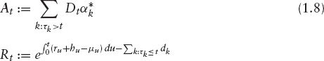
and
![]()
We call X the “pure” stock price process.
The implication of the previous result is that we can focus on the modeling of the pure martingale part X instead of modeling S itself. This will be the subject of this part of the book. Extension to the case of stochastic interest rates or stochastic default intensities is presented in the later chapters of this book.
The previous remarks also allow us to derive the form of the total return version of the stock: Here, we reinvest the proceeds from repo rate and dividends directly back into the asset, as soon as they occur.
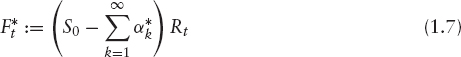
RESULT 2 The total return process S(TR) of the stock is given as
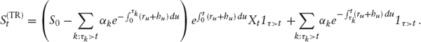
We can also go a step further: Since we are sure of the dividends we will receive, we may forward-sell them. To this end, assume that we buy one share and that we write risky zero bonds for τ1 < τ2< … with notionals ![]() We will be able to honor the respective bond obligations if we reinvest the proceeds from repo rates and continuous dividends into the stock. The gain from forward-selling the dividends will be precisely A0, as defined in (1.8). Hence, the overall price process of this asset is
We will be able to honor the respective bond obligations if we reinvest the proceeds from repo rates and continuous dividends into the stock. The gain from forward-selling the dividends will be precisely A0, as defined in (1.8). Hence, the overall price process of this asset is
The crucial observation is that ![]() is tradable (i.e., available for hedging purposes). This will be used in section 1.4.
is tradable (i.e., available for hedging purposes). This will be used in section 1.4.
Ito in the Presence of Dividends The process (1.6) exhibits jumps, in which case the standard Ito formula does not hold anymore. In our case these jumps are of finite variation, which essentially implies that if we apply Ito to some f ∈ C2, then the second derivative of f will be integrated over the quadratic variation of the “continuous part” of S only. For convenience, let us reformulate (1.6) in terms of purely proportional but then stochastic discrete dividends. To this end we first define the deterministic functions
which are nonzero only on the dividend dates (τk)k=1,…. They represent the fixed and proportional dividends paid at each time t. Accordingly,
We can then define the stochastic “proportional dividend process” by accumulating the cash dividends into the exponential drift of the stock as
![]()
Of course, if there are no fixed cash dividends α, then ![]() is deterministic. The SDE of S can now be written as
is deterministic. The SDE of S can now be written as
where δt(·) denotes the Dirac measure in t. If X is continuous, and if its quadratic variation is absolutely continuous with respect to the Lebesgue measure, then there exists an integrable short-variance process ζ = (ζt)t≥0 and a Brownian motion B such that
![]()
where we have used the Doleans-Dade-exponential
![]()
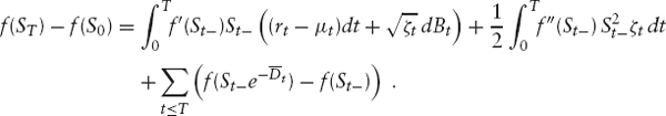
In this case, Ito's formula for S and f ∈ C2 (or finite and convex) becomes
where ![]() is the quadratic variation of the continuous part of S.6 In integral form, (1.14) reads
is the quadratic variation of the continuous part of S.6 In integral form, (1.14) reads
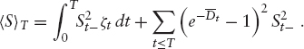
Also note that the quadratic variation of S is given as
1.1.3 European Options on the Pure Stock Process
Since S is an affine transformation (1.6) of the pure stock price X, we can express the prices of European options on the former in terms of prices of European options on the latter. Indeed, let
Then,
where we define
which is the price of call on the pure stock price with strike k.7
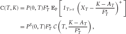
RESULT 3 The call price on a stock S is given in terms of a call C on the pure stock price X as
Hence, if call prices ![]() are available for all strikes and maturities, we can derive the respective prices C(T, k) for all “pure strikes” k from the market via
are available for all strikes and maturities, we can derive the respective prices C(T, k) for all “pure strikes” k from the market via
By put/call parity, the price of a put ![]() on S with strike K and maturity T is given as
on S with strike K and maturity T is given as
![]()
which implies the obvious lower bound
![]()
Consequently, the “pure” put ![]() on X is given in terms of the put
on X is given in terms of the put ![]() on the original stock S as
on the original stock S as
The above results imply that as long as we consider markets where only the stock price process S and European options are liquidly traded, we can focus entirely on the process X. The above equations, (1.17) and (1.18), respectively, allow us to convert one representation into the other. We will frequently switch between the two objects S and X, depending on the application.
1.2 IMPLIED VOLATILITY
The most famous stock price model is the Black & Scholes model. In our framework (1.6), it is given under the unique risk-neutral measure ![]() by assuming that X is a geometric Brownian motion; that is,
by assuming that X is a geometric Brownian motion; that is,
for some non-negative function σ and a ![]() -Brownian motion W. The solution to (1.20) is
-Brownian motion W. The solution to (1.20) is
In fact, this model has been introduced by Samuelson [3] and the time-dependent version above is due to Merton [4], but in practice most people refer to it as the Black-Scholes model (usually in the case without discrete dividends, though). The crucial contribution by Black and Scholes [5] was not so much the model itself, but the fundamental insight that any contingent claim H (ST)) for a sufficiently well-behaved function H can be replicated perfectly by continuous trading in the stock. The impact of this insight cannot be underestimated: Ever since Black and Scholes published their work, a huge industry has evolved in whose core lies the idea of replication of otherwise risky payoffs. The bottom line of the idea is that since we can replicate the payoff, there is no risk in selling a contingent claim. Hence, the costs of replication are certain, and it is justified to call this cost the price of the contingent claim (we will discuss this in more detail in section 1.4).
In the Black-Scholes model, it is particularly easy to compute the prices of many standard payoffs. A standard example is the price of a European call on X with maturity T and “pure strike” k as defined in (1.16) (recall result 3, which shows that it is sufficient to consider X rather than S). Its value is given as
in terms of the famous Black-Scholes formula

To price an option on S in Black and Scholes's framework, note that the price of a call with maturity T and strike K is given as
![]()
Since the Black and Scholes formula ![]() is strictly increasing in σ, it is possible to solve for the latter given a market call price
is strictly increasing in σ, it is possible to solve for the latter given a market call price ![]() (T, k). This yields the common measure of implied volatility for the price of an option:
(T, k). This yields the common measure of implied volatility for the price of an option:
DEFINITION 1.2.1 We call
the implied volatility of X at (T, k) and
![]()
the implied volatility of S for (T, K). Note that by construction ![]() + AT).
+ AT).
Interpretation It should be stressed that the notion of “implied volatility” does not imply that we are actually using the Black-Scholes model. Indeed, it is evident from quoted market prices that their model is no longer sufficient to evaluate contingent claims. To see this, consider figure 1.1, where we have plotted implied volatilities of STOXX50E.8
The effect that implied volatility ![]() is a decreasing function of strike is called skew. Most equity markets have such a shape, but some are less pronounced than STOXX50E; for example, the Japanese N225, which is shown in figure 1.2.9 The point is that implied volatility depends strongly on the strike across all maturities. This means that the underlying stock price process cannot be explained using the Black-Scholes model, for which the implied volatility does not depend on the strike. Rather, we need to find a convenient model for X is able to produce implied volatility surfaces that such as the ones displayed in the figures. When considering alternative models, we should take into account the fact that the general shape of implied volatility is remarkably stable: Figure 1.3 on page 14 shows how the implied volatility surface of STOXX50E has changed in the last few years.
is a decreasing function of strike is called skew. Most equity markets have such a shape, but some are less pronounced than STOXX50E; for example, the Japanese N225, which is shown in figure 1.2.9 The point is that implied volatility depends strongly on the strike across all maturities. This means that the underlying stock price process cannot be explained using the Black-Scholes model, for which the implied volatility does not depend on the strike. Rather, we need to find a convenient model for X is able to produce implied volatility surfaces that such as the ones displayed in the figures. When considering alternative models, we should take into account the fact that the general shape of implied volatility is remarkably stable: Figure 1.3 on page 14 shows how the implied volatility surface of STOXX50E has changed in the last few years.
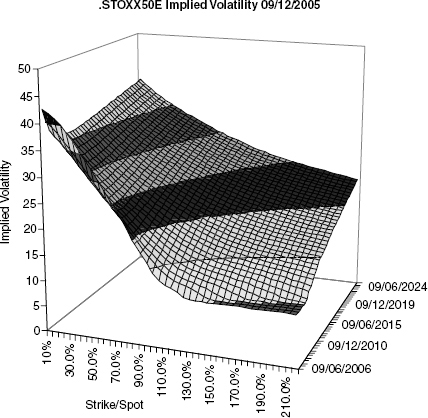
FIGURE 1.1 Implied volatilities for different strikes and maturities for STOXX50E. The graph shows a strong “skew” in strike direction for all maturities.
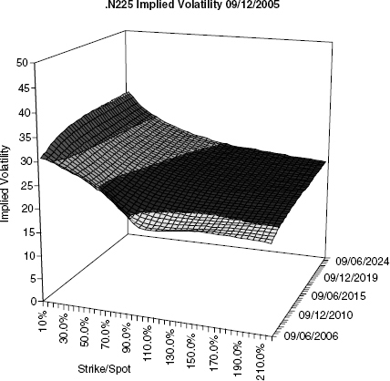
FIGURE 1.2 N225 features nearly a “smile”-type shape in strike.
1.2.1 Sticky Volatilities
Another interesting question is how implied volatility moves on an instantaneous time scale when the stock price moves. Following Balland [6], we consider sticky strike and sticky delta markets. In a sticky strike market, the implied volatility ![]() of an option on S with cash strike K is deterministic. In a sticky delta market, on the other hand, the implied volatility “relative to the forward” or, in our case,
of an option on S with cash strike K is deterministic. In a sticky delta market, on the other hand, the implied volatility “relative to the forward” or, in our case, ![]() , is deterministic. The impact of the actual behavior of the implied volatility can best be seen in the effect on the delta of a European option (for notational simplicity, assume that S = X). To this end, we write the implied volatility
, is deterministic. The impact of the actual behavior of the implied volatility can best be seen in the effect on the delta of a European option (for notational simplicity, assume that S = X). To this end, we write the implied volatility ![]() of S at time t = 0 as a function of S0 as
of S at time t = 0 as a function of S0 as ![]() The price of a call with maturity T and strike K is then
The price of a call with maturity T and strike K is then

FIGURE 1.3 Historic STOXX50E implied volatility during the last few years.
In a sticky strike market, the function ![]() does not depend on S0, that is,
does not depend on S0, that is, ![]() Σ(T, K), for some function Σ. In a sticky delta situation, on the other hand, we have
Σ(T, K), for some function Σ. In a sticky delta situation, on the other hand, we have ![]() Consequently, the total derivative of (1.23) with respect to S0 is
Consequently, the total derivative of (1.23) with respect to S0 is
The symbol ΔBS denotes Black and Scholes's delta (the derivative of ![]() is S0) and the symbol VBS denotes Black and Scholes's vega (the derivative in volatility). In a sticky strike situation, the derivative
is S0) and the symbol VBS denotes Black and Scholes's vega (the derivative in volatility). In a sticky strike situation, the derivative ![]() is zero (i.e., the delta of the call is given as Black and Scholes's delta). In contrast, consider a sticky delta market. In this case, we have
is zero (i.e., the delta of the call is given as Black and Scholes's delta). In contrast, consider a sticky delta market. In this case, we have ![]() Since the slope of implied volatility is typically decreasing, this means that
Since the slope of implied volatility is typically decreasing, this means that ![]() the implied volatility for a fixed cash strike K rises if stock rises (note that it is actually possible to compute the sticky delta purely from market data; cf. remark 2.3.2 on page 78). This is in contrast to market experience: At least for strikes around ATM, an increasing spot level will usually lead to a decline in volatility levels.10 Hence, a sticky delta assumption is not compatible with market behavior.
the implied volatility for a fixed cash strike K rises if stock rises (note that it is actually possible to compute the sticky delta purely from market data; cf. remark 2.3.2 on page 78). This is in contrast to market experience: At least for strikes around ATM, an increasing spot level will usually lead to a decline in volatility levels.10 Hence, a sticky delta assumption is not compatible with market behavior.
Interestingly, both sticky strike and sticky delta behavior of the implied volatility can be characterized neatly following Balland [6]. Under the assumption that the driving stock price is a square-integrable martingale, he shows that the stock price in a sticky delta market must have independent increments, while the only stock price process that is compatible with a sticky strike market is Black and Scholes (i.e., the case without skew).
An intuitive argument for the latter result goes as follows: Assume the market is sticky strike, and that there are two calls with different strikes and the same maturity, each with a different implied volatility. However, only one of the two implied volatilities can actually be realized, which means at least in continuous time processes that only one of the two hedges can work (see also section 2.2.1). (For a thorough derivation of the result refer to Balland [6].)
REMARK 1.2.1 This means that a volatility surface that has skew and is arbitrage free for a given spot value S0 will no longer be arbitrage free for any other spot value.
To see why a sticky delta model implies that the stock price process has independent increments, note that in a sticky delta model, the price of a forward started call with payoff
![]()
for 0 ≤ T1 < T2 is given at time T1 as
![]()
This is a deterministic quantity; hence, the price today of the forward started call is equal to its value at T1 (recall that we have assumed that there are no interest rates). Since it is possible to extract the forward distribution of ST2/ST1 from the forward started call prices by taking their second derivatives, it follows that the stock price has independent increments. Examples of such processes include exponential Levy processes. In contrast, stochastic volatility models such as Heston's (2.1) are not sticky delta because the implied volatility in such models does not move due only to the movement of the spot, but also due to the movement of the other state variables (i.e. the short volatility). Also compare remark 2.3.2 on page 78, where the delta in (very general) stochastic volatility models is computed from the market.
1.3 FITTING THE MARKET
In this section we make the idealizing assumption that European options ![]() (T, k) on X (or S, equivalently) are traded for all strikes and maturities. In such a situation, it is very natural to ask whether the observed market prices are in some way “free of arbitrage” in that they can be reproduced with a martingale that has the required marginal distribution.
(T, k) on X (or S, equivalently) are traded for all strikes and maturities. In such a situation, it is very natural to ask whether the observed market prices are in some way “free of arbitrage” in that they can be reproduced with a martingale that has the required marginal distribution.
1.3.1 Arbitrage-Free Option Price Surfaces
In general, absence of arbitrage proves to be a tricky concept when it comes to continuous time processes. While in discrete time the former is equivalent to the existence to an equivalent martingale measure, this is not true anymore in continuous time, and examples of markets exist, which are free of arbitrage but where not even a local martingale measure exists (the standard reference on this topic is Delbaen/Schachermayer [2]). To avoid technical difficulties, we will therefore introduce a stronger notion of absence of arbitrage:
DEFINITION 1.3.1 We say the market of European call prices ![]() is strongly free of arbitrage if there exists a non-negative true martingale X on some stochastic base
is strongly free of arbitrage if there exists a non-negative true martingale X on some stochastic base ![]() which reprices the market, that is,
which reprices the market, that is,
for all (T, k) ![]()
The key contribution in this context is due to Kellerer [7]:11
THEOREM 1.3.1 The market ![]() is strongly free of arbitrage if and only if
is strongly free of arbitrage if and only if
- (a) For all T, the function
 (T,.) satisfies:
- It is continuous, strictly decreasing and convex in k.
- Its right-hand derivative in k satisfies 0 ≥ ∂k(T, k) ≥ −1.
- (T, 0) = 1 and limk↑∞ (T, k) = 0.12
- For all k, the function (.,k) is increasing.
- (0, k) = (1 − k)+.
The martingale that reprices the market can be chosen to be Markov.
Note that the above conditions allow that ∂k![]() (T,0) > −1. This is the case if the random variable XT has a nontrivial probability mass in zero. Since X is non-negative, the state zero must be absorbing, hence, X can “default” without τ being triggered (which can be interpreted as that the company still serves its debt obligations). However, we regard this as an undesirable property and will understand, if not mentioned otherwise, that ∂k
(T,0) > −1. This is the case if the random variable XT has a nontrivial probability mass in zero. Since X is non-negative, the state zero must be absorbing, hence, X can “default” without τ being triggered (which can be interpreted as that the company still serves its debt obligations). However, we regard this as an undesirable property and will understand, if not mentioned otherwise, that ∂k![]() (T, k) = −1.
(T, k) = −1.
EXAMPLE 1 The “constant elasticity of variance” (CEV) model by Cox [8] is given as the unique strong solution to the SDE
where ![]() .13 This model is occasionally used as a “local volatility” approach to incorporate skew (the resulting implied volatility exhibits an upward-sloping downside skew).
.13 This model is occasionally used as a “local volatility” approach to incorporate skew (the resulting implied volatility exhibits an upward-sloping downside skew).
For all β < 1, the process X can reach zero with a nonzero probability and then “dies” there.
Theorem 1.3.1 is a convenient tool to assess whether a given market or an interpolation scheme for market prices is free of strong arbitrage. However, it does not describe how the process X can actually be computed. The best-known approach in this direction is Dupire's “implied local volatility” for continuous market price processes, which requires the knowledge of European option prices for all strikes and maturities. Madan/Yor discuss alternatives to construct pure jump processes [10]. For the discrete case where only a finite number of European options is provided, time and state discrete martingales can also be constructed, as we will show below.
1.3.2 Implied Local Volatility
The core idea of implied local volatility is due to Dupire [11]. His idea is intriguingly simple: Given observed market prices ![]() (T, k) for all
(T, k) for all ![]() and
and ![]() we ask: is it possible to find a function
we ask: is it possible to find a function ![]() such that the solution to the SDE
such that the solution to the SDE
![]()
for a Brownian motion W exists, is unique, has the martingale property, and reprices the market? That this is indeed possible can be derived using the following theorem due to Gyöngy [12] (the original work [11] used an approach via the Fokker-Planck equation):
THEOREM 1.3.2 If Y is an m-dimensional continuous semi-martingale of the form
with predictable bounded and integrable drift α and volatility matrix β, then the solution to
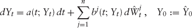
with
![]()
exists, is unique, and has the same marginal distributions as ![]()
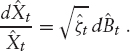
Let us assume that the “real market” price process ![]() is a true strictly positive martingale under some measure
is a true strictly positive martingale under some measure ![]() . In this case (and if the quadratic variation of the stock is absolutely continuous with respect to the Lebesgue measure),14 there exists a
. In this case (and if the quadratic variation of the stock is absolutely continuous with respect to the Lebesgue measure),14 there exists a ![]() -Brownian motion
-Brownian motion ![]() and a stochastic “short variance” process
and a stochastic “short variance” process ![]() such that
such that ![]() satisfies
satisfies
The market price of a call with strike k and maturity T is then given as
![]()
Theorem 1.3.2 implies that given some Brownian motion B on some stochastic base, the SDE
![]()
with
![]()
has a unique strong solution which has the same marginal distribution as ![]() . Therefore, X reprices all European options; in particular,
. Therefore, X reprices all European options; in particular, ![]() for all t (i.e., X is a true martingale).
for all t (i.e., X is a true martingale).
To obtain an analytic form for σ, we use Ito's formula for convex payoffs:

Taking expectations and derivation in T yields
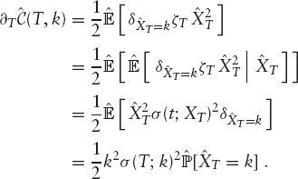
Since the density of ![]() can be computed as
can be computed as ![]() we obtain Dupire's formula: given
we obtain Dupire's formula: given
the unique solution X to
exists, is a martingale, and reprices the market. An example can be found in figure 1.4.
REMARK 1.3.1 The above formula is given in terms of the calls on the pure stock price ![]() . This is much more robust than using the call prices on
. This is much more robust than using the call prices on ![]() via (1.18) since the effect of discontinuities in the forward (resulting from discrete dividends) are eliminated.
via (1.18) since the effect of discontinuities in the forward (resulting from discrete dividends) are eliminated.
It is also possible to write (1.26) in terms of implied volatility (which has the same advantage of being robust with respect to jumps in the forward, etc). To this end, one simply replaces the call prices in (1.26) by their equivalent values in terms of the Black and Scholes formula and the implied volatilities.
Conceptually, implied local volatility is a very neat approach: starting from the observable implied distribution of the underlying martingale ![]() , a diffusion X is constructed that has the same marginal distributions as the original process.
, a diffusion X is constructed that has the same marginal distributions as the original process.

FIGURE 1.4 Implied volatility and implied local volatility of SPX. The local volatility is computed using Dupire's formula and then interpolated by a smooth spline.
This approach ensures that the resulting process X reprices all European claims correctly. In particular, skew exposure for European knock-out options and the like is taken into account properly: as an example, consider a European digital call that pays 1 if the stock is above the strike at maturity. The impact of skew on such a product is severe. The graph in figure 1.5 shows the difference between plain BS prices (computed with the strike-implied volatility) and the local volatility price. We have also provided the price given by a tight call spread, ![]()
![]()
The issue with (1.26) in practice is that it is very difficult to be used directly. The main problem is that we usually have only a finite number of traded European options. In order to obtain a local volatility function using Dupire's formula (1.26), we therefore need to intra- and extrapolate option prices (or implied volatilities). The resulting European call price surface then needs to satisfy the no-arbitrage conditions of theorem 1.3.1 to ensure that (1.26) is finite and not imaginary. Moreover, the volatility function σ itself must ensure that the solution to (1.27) is unique and nonexplosive.15 This is highly nontrivial and makes an extra- and interpolation algorithm for discretely quoted market prices difficult to implement in practice. A far more robust approach is calibration of a local volatility function via forward PDEs, as described in chapter 8.
EXAMPLE 2 Assume that market price process is a “jump diffusion” (cf. Merton [14])
where N is a Poisson process with intensity h and where ξ = (ξi)i is an iid sequence of random variables independent of N with a nontrivial distribution; moreover, ![]() The process W is a Brownian motion and σ is a constant.
The process W is a Brownian motion and σ is a constant.
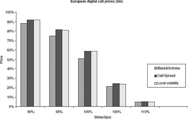
FIGURE 1.5 The prices of digital options for various strikes, computed with the Black-Scholes model, by approximation via call prices and by using implied local volatility. The example shows the importance of capturing the skew correctly when pricing nontrivial European options.
In this case, (1.26) is not well defined at T =0; hence, no solution to the problem of fitting the market with a diffusion of the type (1.27) exists.
1.3.3 European Payoffs
While implied local volatility is a very valuable tool to price path-dependent options, nonvanilla European options by themselves can be priced more straightforwardly by using directly quoted vanilla options.
To this end, note that any twice differentiable function H: ![]() can be written as
can be written as
that is, as long as we can trade European options ![]() and
and ![]() with all strikes at the maturity T, and under suitable integrability assumptions, we can compute
with all strikes at the maturity T, and under suitable integrability assumptions, we can compute
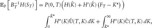
which holds for any potential martingale measure ![]() and also covers the possibility of default where the payoff at maturity is H(0). The strike
and also covers the possibility of default where the payoff at maturity is H(0). The strike ![]() is arbitrary and can be set to the forward. Note that (1.29) also holds for convex functions with their generalized derivatives. In particular, H does not need to be defined in 0: for example, the formula is also valid for the convex function H (x) = x − 1 − log (x), the price for which is infinite if the stock has a nonzero probability of default.
is arbitrary and can be set to the forward. Note that (1.29) also holds for convex functions with their generalized derivatives. In particular, H does not need to be defined in 0: for example, the formula is also valid for the convex function H (x) = x − 1 − log (x), the price for which is infinite if the stock has a nonzero probability of default.
The advantage of using (1.29) instead of implied local volatility to price the payoff H is that (1.29) also yields a hedge for H: by construction, the formula will tell us how many European options of each strike we have to buy to perfectly replicate the payoff H. This is of great advantage, since an implied local volatility model in itself gives a hedging strategy only in terms of the spot (cf. section 1.4). Of course, in practice we will neither be willing nor able to invest in infinitely many options. Instead, we will limit ourselves to a reasonable discretization of the real line. The first step is to super-replicate H; we concentrate on convex functions since most financial payoffs are convex functions or combinations thereof.
A convex function H can be approximated from above by linear functions. That means that if we select two sequences ![]() and
and ![]() of strikes with
of strikes with ![]() and
and ![]() respectively, then an approximation
respectively, then an approximation ![]() of H from above,
of H from above, ![]() is given by
is given by
with

and

A similar formula holds for a subreplication strategy.
If H is a function that is finite in zero and linear beyond some K* in the sense that H[K*,∞)(x) = αx + β, we can use only a finite number of strikes: the corresponding super-replicating payoff is given by

where ![]() The condition that H is linear beyond some strike is necessary to be able to limit ourselves to some maximal strike. Alternatively, we could postulate that for some large strike K*, the value of the respective call is practically zero, and will remain zero for the life of the contract we want to price. We hence assume that there is no probability mass beyond this “zero price strike” K*. Then, (1.31) gives a super-replication price and indeed a super-hedging position for all convex payoffs.
The condition that H is linear beyond some strike is necessary to be able to limit ourselves to some maximal strike. Alternatively, we could postulate that for some large strike K*, the value of the respective call is practically zero, and will remain zero for the life of the contract we want to price. We hence assume that there is no probability mass beyond this “zero price strike” K*. Then, (1.31) gives a super-replication price and indeed a super-hedging position for all convex payoffs.
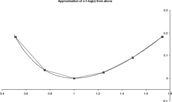
FIGURE 1.6 The super-hedge for the function H (x) := x − 1 − log (x).
Interpretation It should be noted that this approach is tantamount to assuming that the stock price will attain only discrete values in T, namely the strikes ![]() this is because (1.30) is nothing but the price of H computed under the probability measure
this is because (1.30) is nothing but the price of H computed under the probability measure
where
![]()
(recall from (1.24) that ![]() are the market prices of calls on X). It is an attractive idea because it will always compute an upper bound for convex payoffs. Accordingly, we call a stock price model with (1.32) a “most expensive” model. Since the assumptions made (such as the existence of K*) are relatively weak, it provides a good framework to assess the value of a European payoff H (of course pricing via (1.32) is not limited to convex payoffs). If we want to follow this approach for options that depend on more than one maturity, though, we also have to construct the transition probabilities between the marginal distributions (1.32). This is the subject of the next section.
are the market prices of calls on X). It is an attractive idea because it will always compute an upper bound for convex payoffs. Accordingly, we call a stock price model with (1.32) a “most expensive” model. Since the assumptions made (such as the existence of K*) are relatively weak, it provides a good framework to assess the value of a European payoff H (of course pricing via (1.32) is not limited to convex payoffs). If we want to follow this approach for options that depend on more than one maturity, though, we also have to construct the transition probabilities between the marginal distributions (1.32). This is the subject of the next section.
1.3.4 Fitting the Market with Discrete Martingales
We will now discuss an alternative to implied local volatility which follows the construction (1.32) above. The idea here is not to assume that a smooth surface of European option prices is quoted in the market, but to give in to the fact that many of these options are traded only finitely. We saw in the previous section that such an assumption implies that we can replicate European payoffs using the liquid vanilla instruments. The same will not hold true if we construct transition densities between the marginal distributions (1.32), because these transition densities are not uniquely defined by the observable market prices. However, following Buehler [16], we will give a constructive approach identifying suitable transition matrices by imposing “secondary information.” More precisely, we will choose kernels that match the prices of more exotic payoffs such as forward started options.
To be precise, assume that a discrete number of call prices ![]() can be observed in the market; we denote by T the set of maturities for which we have at least one call price, and we enumerate them as 0 ≤ T1 < … < Tm. For each maturity Tj, we denote by Kj := {k: (Tj, k) ∈ A} the set of strikes for which calls are quoted. To avoid the case of local martingales we assume that 0 ∈ Kj with
can be observed in the market; we denote by T the set of maturities for which we have at least one call price, and we enumerate them as 0 ≤ T1 < … < Tm. For each maturity Tj, we denote by Kj := {k: (Tj, k) ∈ A} the set of strikes for which calls are quoted. To avoid the case of local martingales we assume that 0 ∈ Kj with ![]() (Tj, 0) = 1. We also assume as in the previous section that there is some (artificial and large) “zero price” strike k* ∈ Kj such that
(Tj, 0) = 1. We also assume as in the previous section that there is some (artificial and large) “zero price” strike k* ∈ Kj such that ![]() (Tj, k*) = 0 for all j. To ease notation, we write
(Tj, k*) = 0 for all j. To ease notation, we write ![]() for the strikes of calls with maturity τj. We will also make use of the first differences,
for the strikes of calls with maturity τj. We will also make use of the first differences,

for ![]() = 0, …, dj − 1 and
= 0, …, dj − 1 and ![]() Finally, we will also need the lower convex hull of all call prices beyond some maturity, that is,
Finally, we will also need the lower convex hull of all call prices beyond some maturity, that is,
![]()
Note that this function is just the lower convex linear hull of all call prices with maturities Ti with i > j.
The following corollary is a direct consequence of theorem 1.3.1:
COROLLARY 1.3.1 The discrete set of call prices ![]() is strongly free of arbitrage if, and only if, the following conditions hold:
is strongly free of arbitrage if, and only if, the following conditions hold:
- Convexity: For all j = 1, …, m,

- Monotonicity: For all j = 1, …, (m − 1) and all k ∈ Kj,
![]()
In particular, there exists a non-negative martingale X with states Kj per maturity Tj with a marginal distribution given by
for ![]() = 0,…,dj.
= 0,…,dj.
If, in addition, ![]() then X is strictly positive.
then X is strictly positive.
It is quite straightforward to check these conditions for real market data. (In Buehler [16], it is also discussed how to turn data that do not satisfy the above conditions into a “close” fit which then satisfies the conditions.) The crucial point is that we can actually construct a martingale X as described in the above corollary. Before we discuss this, let us recall from the discussion in section 1.3.3 that all martingales that realized a density (1.33) are “most expensive” in the following sense: Let Y on ![]() be any other martingale (possibly with continuous state space and time) which reprices the market, that is, for all j = 1, …, m and kj ∈ Kj we have
be any other martingale (possibly with continuous state space and time) which reprices the market, that is, for all j = 1, …, m and kj ∈ Kj we have
![]()
Then X is more expensive than Y for any convex payoff ![]() that is,
that is,
![]()
for all j = 1, …, m.
Constructing Discrete Transition Densities Let us now denote by ![]() the row vector of probabilities of XTj being exactly
the row vector of probabilities of XTj being exactly ![]() that is,
that is,
![]()
for ![]() = 1, …,dj and
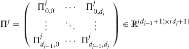
= 1, …,dj and ![]() For any discrete martingale X with states Kj at maturity Tj, there exists a transition kernel
For any discrete martingale X with states Kj at maturity Tj, there exists a transition kernel
with transition probabilities ![]() “from
“from ![]() to
to ![]()
![]()
Hence, the problem at hand is how to find a sequence of kernels (Πj)j=1, …, m such that
![]()
for all j = 1, …, m. More precisely, we search for a sequence of matrices (Πj)j for which the following properties hold:
- Each element of Πj is non-negative.
- Each row of Πj is a probability distribution,16
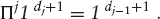
- Πj has the martingale property, that is, for
 we have

- Πj is compatible with the marginal distributions,
![]()
The key is now that the above conditions (a)–(b) are all linear in the coefficients of Πj. That implies that we can formulate the quest for Πj as a linear programming problem,
where πj is the vector of all elements of Πj and where ![]() and
and ![]() (two of the linear conditions are redundant). For such problems, very efficient algorithms exist, and we can solve even large systems very quickly; the existence of a solution is guaranteed by corollary 1.3.1. Note that this means that the space of solutions for (1.34) is very large—while the number of elements of π grows quadratically, the number of conditions grows only linearly. This simply reflects the fact that many possible transition densities are compatible with the observed marginal distributions.
(two of the linear conditions are redundant). For such problems, very efficient algorithms exist, and we can solve even large systems very quickly; the existence of a solution is guaranteed by corollary 1.3.1. Note that this means that the space of solutions for (1.34) is very large—while the number of elements of π grows quadratically, the number of conditions grows only linearly. This simply reflects the fact that many possible transition densities are compatible with the observed marginal distributions.
To put it positively, this means that we can select a transition kernel that satisfies “secondary requirements.”
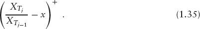
Repricing Forward Started Options Any of the solutions to (1.34) will perfectly reprice the observed European option prices. However, it is often desirable also to impose certain assumptions on the prices of forward started options: a fixed strike forward started option with “reset date” T1 and maturity T2 > T1 has the payoff
![]()
While it is trivial to compute the value of such a payoff in the Black-Scholes model, it is by far not clear what the fair value of such a contract should be in the market. We will come back to this type of product at a later stage in section 2.1.6. Here, we assume that we have a good idea of the price of a few strikes for each of the options between Tj−1 and Tj. Accordingly, we denote by ![]() j(x) the price of an option with payoff
j(x) the price of an option with payoff
Its price given a transition kernel Πj is
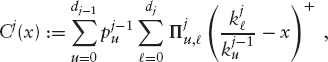
which is once more just a linear expression in the elements of Πj. The idea is now to choose a transition kernel Πj, which minimizes for a range x1 < … < xn of strikes the distance between model prices and assumed market prices, that is,
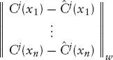
under an appropriate norm. This leads to an optimization problem of the form

For w = 1 and w = ∞, this reduces again to linear programming. For w = 2, it is a linear least-squares problem, which can also be solved efficiently.17
Pricing and Hedging In a model with discrete states, it is straightforward to evaluate options whose value depends only on the dates T1, …,Tm. A discrete-state Monte Carlo engine, for example, just needs to invert the conditional transition probabilities, which can be accomplished very efficiently; cf. Glasserman [17]. For multi-asset applications, an ad hoc approach is to use copulas to model their interdependency (see chapter 7). The method lends itself also to backward pricing, since the necessary (expensive) inversion of the transition matrices needs to be done only once during the life of the model.
1.4 THEORY OF REPLICATION
In section 1.3.2, we introduced the concept of implied local volatility, where the pure stock price process X under a martingale measure ![]() is given as
is given as
for a function σ, which can in theory be implied from market quotes of European prices. One striking feature of such a model is that it is generally complete: we can replicate the payoff of an option by continuous trading in the stock. This is in stark contrast to the discrete model above, where such a strategy except for European payoff is not available.
Replicating Trading Strategies To illustrate the idea of replication, assume that we sell a European claim with payoff18
![]()
To ease notation in the following, we will concentrate solely on the case of zero dividends, default probability, and interest rates (i.e., on the case where S = X). We comment on the general case afterward.
The question is now the following: Can we trade in X such that the result of trading plus a potential initial capital has at T the same value as HT? This requires the concept of a trading strategy: a trading strategy Δ = (Δt)t∈[0, T] is a (random) process whose value Δt denotes the amount of shares we should hold at time t. This value may depend on past information, in particular the path of X up time t, but it obviously cannot include any future information of the value of X. Mathematically, we say that the process Δ must be predictable. We also require that the process is suitably integrable (i.e., ![]() is almost surely finite) and bounded from below.19
is almost surely finite) and bounded from below.19
To execute the trading strategy, assume we have an initial capital of H0 and that we start at time 0 with buying Δ0 shares. We borrow the required amount C0 = Δ0X0 − H0 from the bank,20 so that the value of our portfolio at time 0 is V0 = H0.
Let us consider first discrete time trading, that is, that the hedging strategy Δ is constant on intervals [(k − 1)τ, kτ] for k = 1, …, n with τ := T/n, i.e. nτ = T. After the end of the first interval, the value of our position in X has changed due to the movement of the stock (i.e., it is now Δ0Xτ), while our debt of Δ0X0 − H0 did not change since we assumed that interest rates are zero. Now we rebalance our position in X according to our hedging strategy, which tells us now to hold Δτ units of X. Accordingly, we have to buy (Δτ − Δ0) shares for the price of (Δτ − Δ0)Xτ, the excess of which we need to borrow again from the bank. The overall cost to hold Δτ shares in τ is therefore
![]()
Proceeding further in time, the accumulated cost to hold Δkτ at time kτ is

The value of our portfolio including the shares is

In case of a continuous trading strategy, the same arguments hold: the right hand sum converges against the integral of Δ over X, so we have
![]()
for all t ∈ [0, T]. We now call the strategy Δ replicating, if the value of VT matches the value of HT, that is, if
The point here is that the cost of replicating HT is covered by the constant H0, which justifies calling it the fair price of HT. If such a replication strategy is possible for all payoffs of some set X, then we say that the market (X, X) is complete.21
The most natural market X is what we call the market of relevant payoffs: assume we are allowed to trade in X and in some liquid instruments C = (C1, …, Cn). Then the only economically relevant payoffs are those that depend functionally on X and C; this means that we will consider only payoffs that are measurable with respect to ![]() for some finite T (in contrast to payoffs measurable with respect to the larger σ-algebra FT). As usual, we also limit ourselves to payoffs that are bounded from below. We now simply say the market (X, C) is complete, if any payoff HT that is measurable with respect to FX, C and bounded from below can be replicated by some trading strategy (Δ, φ)22 in the sense that
for some finite T (in contrast to payoffs measurable with respect to the larger σ-algebra FT). As usual, we also limit ourselves to payoffs that are bounded from below. We now simply say the market (X, C) is complete, if any payoff HT that is measurable with respect to FX, C and bounded from below can be replicated by some trading strategy (Δ, φ)22 in the sense that
Of course, it is generally not clear that such a replication strategy exists—the reason why replication works in a local volatility model is that we have assumed that there is an equivalent measure ![]() under which the process X, defined by equation (1.37), is a Markovian martingale. To this end, consider now again a payoff HT ≡ H(XT) given in terms of a smooth, bounded function H with bounded derivatives. We can then define, somewhat ad hoc, the bounded martingale (Ht)t∈[0, T]
under which the process X, defined by equation (1.37), is a Markovian martingale. To this end, consider now again a payoff HT ≡ H(XT) given in terms of a smooth, bounded function H with bounded derivatives. We can then define, somewhat ad hoc, the bounded martingale (Ht)t∈[0, T]
![]()
Because of the Markov-property of X, this can be written as
![]()
If we assume that h is a C1,2 function, we can apply Ito and find, using the martingale property of Ht, that
![]()
Hence, we have found a trading strategy Δt := ∂Xht(Xt), which replicates our payoff, and the price ![]() Similarly, at any later time t < T, we can write
Similarly, at any later time t < T, we can write
![]()
that is, the value Ht is the fair price of HT at t.
1.4.1 Replication in Diffusion-Driven Markets
The above considerations can now also be applied to more general cases: we will now show how hedging works in a framework where a range of market instruments is driven by an underlying Markov process (we will concentrate on diffusions here). This will be put to use in section 2.3 when we discuss hedging of options on variance with variance swaps. The idea is as follows: if we want to hedge a payoff HT ≡ H(XT), we will try to use the stock price X to hedge it, but if the market is not a local volatility model, we will need additional traded instruments to cover us against changes in the value of HT. To this end, we assume that there are liquid instruments C = (C1, …, Cn) that are traded alongside the stock. For example, think of a finite number of European options on S. We assume without loss of generalization that the price processes ![]() for
for ![]() = 1, …, n are defined until T; for an option with an earlier maturity T* < T, we simply set
= 1, …, n are defined until T; for an option with an earlier maturity T* < T, we simply set ![]() for t ∈ [T*, T]. We also assume that C1, …, Cn are bounded from below.
for t ∈ [T*, T]. We also assume that C1, …, Cn are bounded from below.
To apply the same idea as for the case of local volatility, we now stipulate that the vector (X, C1, …, Cn) of market instruments is given in terms of a finite-dimensional diffusion Z = (Zt)t∈[0, T] with open state space ![]() by a function
by a function ![]() as
as
![]()
The function ![]() is assumed to be invertible and differentiable. For all applications it will be appropriate to assume that X itself is among the state variables Z, and we set Z0 := X accordingly. The process Z is thought to represent the “state factors” of the market. The inherent assumption is that the relevant information available in the entire market is incorporated in a finite set of states Z; in the end, we could well assume that Z = (X, C1, …, Cd), but it is often tricky to model, say, European options along with the stock price.
is assumed to be invertible and differentiable. For all applications it will be appropriate to assume that X itself is among the state variables Z, and we set Z0 := X accordingly. The process Z is thought to represent the “state factors” of the market. The inherent assumption is that the relevant information available in the entire market is incorporated in a finite set of states Z; in the end, we could well assume that Z = (X, C1, …, Cd), but it is often tricky to model, say, European options along with the stock price.
We limit our attention to diffusions and assume that Z is the unique strong solution to an SDE
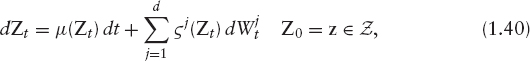
where W = (W1, …, Wd) is a d-dimensional Brownian motion. The drift vector μ = (μ0, …, μm): ![]() and the volatilities
and the volatilities ![]() for are not explicitly time dependent, but imposing, say, zm := 0, μm := 1 and
for are not explicitly time dependent, but imposing, say, zm := 0, μm := 1 and ![]() allows to set
allows to set ![]()
Note, in particular, that in contrast to standard assumptions, we do not require that ζ has full rank. We merely require that the SDE (1.40) has a unique strong solution. A sufficient but not necessary criterion is that μ and ζ are Lipschitz continuous.
EXAMPLE 3 Let

such that ζ is well defined and set Zt := (Xt, ζt, t). Such a model satisfies the above assumptions with
![]()
where ![]() is the value of a European option with maturity T* ≥ T, for example,
is the value of a European option with maturity T* ≥ T, for example,
![]()
EXAMPLE 4 In the same setting as in the example before, define Z0 := X, Z1 := ζ, ![]() and, additionally,
and, additionally, ![]() see also section 2.3. Then,
see also section 2.3. Then,
satisfies the assumptions made before. The contract C1 is called the variance swap with maturity T on X. We will see in section 2.3 that these instruments are very natural hedging instruments for options on realized variance.
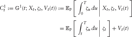
Delta Hedging Works Now assume as before that we want to hedge a smooth, bounded European payoff HT = H(XT). As before, we define the martingale (Ht)t∈[0, T] via
![]()
Note that because we have assumed that H is bounded, this is a true martingale. Using the Markov property of Z, we can write again
![]()
Since ![]() is invertible, we can set
is invertible, we can set ![]() such that given X and C = (C1, …, Cn), we have
such that given X and C = (C1, …, Cn), we have
![]()
ASSUMPTION 1 For smooth-bounded functions ![]() with bounded derivatives and compact support, the function
with bounded derivatives and compact support, the function
![]()
is C1 in z for all t and continuous in t.
If the assumption holds, then h is differentiable in z, and so is g (via the inverse function theorem applied to ![]() ). An application of Ito (possibly to an approximation of g by C1,2 functions)23 shows that “delta hedging works,”
). An application of Ito (possibly to an approximation of g by C1,2 functions)23 shows that “delta hedging works,”

General Contingent Claims To handle more general payoffs, note that we can approximate nonsmooth European payoffs by bounded smooth payoffs, and that general path-dependent payoffs of the form HT = H(Xt∈[0, T], Ct∈[0, T]) can be approximated by payoffs that depend on finitely many states of X and C. The latter payoffs, in turn, can be approximated by payoffs that are products of payoffs of the form Hk(Xtk, Ctk) for a finite number of dates t1, …, tn′; see also [18]. The crucial condition to ensure completeness of the market is that assumption 1 holds.
THEOREM 1.4.1 Under assumption 1, the market of relevant payoffs on (X, C) is complete.
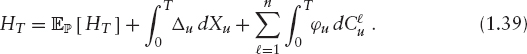
For example, option payoffs with prices Ht = ht(Zt, At), which depend not only on Z, but on some finite variation process A = (A1, …, Aq) can be still delta-hedged with Z,

where ![]()
Deterministic Dividends, Interest Rates, and Default Risk Until now, we have focused solely on the case where S = X, that is, we have abandoned the deterministic market data of the first section. Let us briefly comment on the impact of using
![]()
according to (1.6). The aim is to replicate H(ST).
As a first step, we distinguish between default and no default. Since S drops to zero upon default,
![]()
Hence,

with ![]() Since we can lock in (P(0, T) − PS(0, T)) H(0) by entering into a static position of risky and riskless bonds, we need to concentrate only on the replication of
Since we can lock in (P(0, T) − PS(0, T)) H(0) by entering into a static position of risky and riskless bonds, we need to concentrate only on the replication of ![]() We hence define
We hence define
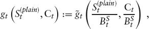
As before, we assume that Z = (Z0, …, Zm) with Z0 = X is uniquely given by the SDE (1.40), and that a range of traded instruments C = (C1, …, Cn) is given as a function of Z. Without loss of generality we can assume with the same trick as above that each instrument C![]() attains zero value upon default; hence, we set
attains zero value upon default; hence, we set
![]()
We will also strip S of all its dividends and the repo by using the (tradable) process S(plain) defined in (1.9). The key is that we will use the risky bond BS as the cash account, that is, we aim to construct a replication strategy such that
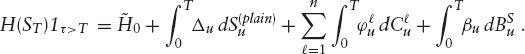
As usual, the value of β is determined on the set {τ > t} by the self-financing requirement as

The next step is to express, as before, the conditional expectation (1.43) in terms of Z, rewrite it by the invertibility assumption in terms of C, and then apply Ito. Let ![]() and
and ![]() to which our previous results apply if g is sufficiently smooth. Defining, moreover,
to which our previous results apply if g is sufficiently smooth. Defining, moreover,
yields that on {τ > t},

In other words, the market is complete.
1 Section 9.6 on page 279 covers the pricing of convertible bonds under various more detailed assumptions.
2 Blanchet-Scalliet/Jeanblanc [1] provide a good introduction into intensity models.
3 Mathematically speaking, an accessible stopping time can be approximated by an increasing sequence of stopping times (τn)n with τn ↑ τ for n ↑ ∞.
4 We implicitly assume that we by ourselves cannot default.
5 The notion of “no free lunch with vanishing risk” is a stronger form of “no arbitrage.” Only the former is equivalent to the existence of a local martingale measure, and we will always assume we are in this setting. See Delbaen/Schachermayer [2] for a detailed analysis and examples.
6 If f is finite and convex, f″ exists as a positive measure. For example, the second derivative of f(x) := x+ is the Dirac measure in zero, δ0.
7 Strictly speaking, we can call C(T, k) only then the price of the respective call on X, if either the market is complete (i.e., ![]() is unique) or if the call on S with strike
is unique) or if the call on S with strike ![]() and maturity T is quoted in the market, in which case its price is given under any
and maturity T is quoted in the market, in which case its price is given under any ![]() -equivalent martingale measure by (1.15).
-equivalent martingale measure by (1.15).
8 We refer to underlyings by their Reuters code.
9 Symmetric “smiles” are a common feature in FX markets. In other markets, such as commodities, the skew might actually be upward sloping.
10 It can also lead to increase in the skew for downside strikes, hence out-of-the-money put implied volatilities may actually rise.
11 See Föllmer/Schied [9] for a proof.
12 The condition that ![]() (T,0) = 1 ensures that any process with the correct marginals is a true martingale.
(T,0) = 1 ensures that any process with the correct marginals is a true martingale.
13 For ![]() equation (1.25) has infinitely many solutions.
equation (1.25) has infinitely many solutions.
14 Cf. propositions 3.8 (p. 202) and 1.5 (p. 328) in Revuz/Yor [13].
15 A sufficient condition for the existence of a global unique solution to (1.27) is Lipschitz continuity; see Protter [15].
16 We used 1n to denote the unit vector in ![]()
17 Other methods of selecting an appropriate transition kernel include the use of a “mean variance” criterion (which is also linear in the underlying probabilities). See [16] for more details.
18 For technical reasons, assume that H is bounded from below.
19 This excludes the “suicide strategy”: double your bets until you lose.
20 Borrowing a negative amount means to invest it in the bank.
21 It is an important point that the notion of a “fair price” implies the existence of a replication strategy. In incomplete markets, for example, some payoffs cannot be replicated, and therefore do not have a unique price.
22 With ![]()
23 Technical details and tighter results can be found in Buehler [18].