
CHAPTER 8
Forward PDEs and Local Volatility Calibration
8.1 INTRODUCTION
8.1.1 Local and Implied Volatilities
In the Black-Scholes model ([134]), the stock price follows geometric Brownian motion with a constant volatility σ:
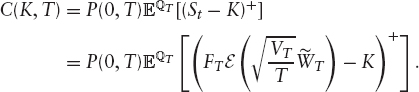
where rt is the short interest rate and νt contains the repo rate and a dividend yield. This is discussed in more detail in chapter 1. Under this assumption, the price of a European call option with strike K and maturity T is given by the Black-Scholes formula
![]()
where P(t, T) is the price at time t of a zero-coupon bond with maturity T, FT is the stock forward, and

Now that the European options themselves form a liquid market, prices are available for many options on many stocks and indices. The implied volatility of an option is the constant volatility that when used in the above equations recovers the market price of the option. Figure 8.1 shows the dependence of the implied volatility of the Stoxx50 index on the maturity and strike of the options.
Since the implied volatility is a function of the strike price, the volatility that we use in equation (8.1) cannot be constant. If we want our stock model to be Markovian in just one factor, we must make the volatility of the stock a deterministic function of both the stock price and time. This is referred to as the local volatility. In reality, though, there is not such a simple relationship between volatility and stock price. Studies of historical market data show that the volatility is stochastic and can be modeled well by mean-reverting processes such as Heston's model [135].

FIGURE 8.1 Implied volatility surface for the Stoxx50 index.
A local volatility model has the benefit over a stochastic volatility model that it is Markovian in only one factor (and therefore more tractable). It is also possible to calibrate a local volatility model to a complete implied volatility surface (assuming there is no arbitrage). It has the drawback that it predicts unrealistic dynamics for the stock volatility and therefore the implied volatility surface. However, a local volatility model is sufficient for pricing some products—particularly ones with European payoffs, which can be hedged perfectly with a static set of positions in European calls and puts.
In a simple one-factor model with no extra sources of randomness, Dupire [136] showed that we can express a local volatility in terms of the implied volatility surface and its derivatives. However, this formula can be difficult to use in practice. If we add more sources of randomness to our model—for example, stochastic interest rates, hazard rates, or dividends—Dupire's formula no longer applies and we must find another way to create a local volatility surface from an implied volatility surface.
Tied in with the problem of calibrating a local volatility surface is the problem of pricing options with European payoffs (where the payoff depends on the value of the stock on a single maturity) where no closed form solutions exist. This can obviously be done by Monte Carlo simulation or backwards induction using a tree or numerical PDE solver. However, simulation methods suffer from a slow rate of convergence, while backward PDE methods and trees have better convergence but can price only one option at a time.
In this chapter, we demonstrate the powerful technique of using forward PDEs to price multiple European options very efficiently. We then go on to discuss how to use this technique to calibrate a local volatility surface to an implied volatility surface in single- and multifactor models.
8.1.2 Dupire's Formula and Its Problems
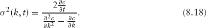
Dupire [136] showed that the local volatility (which we shall denote by σl) can be expressed in terms of the implied volatility surface, or more simply in terms of European call prices. We derive his full result in section 8.3, equation (8.18), but for the purposes of this section, we can ignore the effects of interest rates and dividends.
Letting rt = νt = 0, Dupire's formula becomes
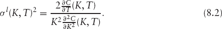
The drawback of this equation in practice is that it requires the knowledge of call prices for all strikes and maturities, whereas in reality there will be data for only call prices at a discrete set of strikes and maturities. We must therefore interpolate the call prices (or implied volatilities) between the market data points if we are to use equation (8.2). For the local volatility to be continuous in the stock price (which is necessary for good convergence of any numerical scheme) we need the second derivatives of the call prices with respect to strike to be continuous. We also need the call prices to be once differentiable with respect to time. Additionally, the call prices must obey the following no-arbitrage conditions:
and
![]()
as well as the boundary conditions
![]()
and
![]()
The equivalent conditions when expressed in terms of implied volatilities are even more complicated to evaluate.
Occasionally, the market data may include regions of arbitrage owing to large bid-offer spreads on illiquid options or the difficulty of extrapolating into regions where there is no data. However, it is necessary to remove all arbitrageability from the implied volatility surface as Dupire's formula is only valid up to the first time when the above conditions are violated. If, instead of trying to fit a smooth implied volatility surface to a discrete set of European options, we assume a local volatility surface σl(S, t), then our arbitrage and boundary conditions become that σl(S, t) is greater than zero and Sσl(S, t) is Lipschitz continuous [137]. Finding a local volatility surface that satisfies these no-arbitrage conditions is much simpler than finding an implied volatility surface. The only difficulty is how to fit the local volatility surface to the market call prices, and this will be addressed in the rest of the chapter.
8.1.3 Dupire-like Formula in Multifactor Models
Another reason for looking for an alternative to Dupire's formula is that to the authors’ knowledge there is no equivalent formula in higher-dimensional models.
To demonstrate the difficulty of finding a two-factor version, we can consider a simple non-dividend-paying stock with interest rates following the Hull-White model [61]. We have

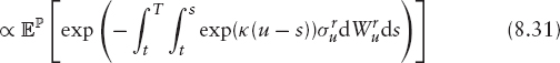
Borrowing equation (8.33) from section 8.6, we have
![]()
(see section 8.6 for details). The local volatility at time T depends not just on the implied volatility and its derivatives at T, but also on the implied volatility at all times t < T. We cannot then hope to find a simple expression like Dupire's formula, even in the simplest case we can study.
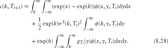
When we follow the steps that lead to Dupire's formula, but with stochastic interest rates (see section 8.4), we arrive at the following expression (see equation (8.27)):

where c, x, y, and k are transformed call prices, stock prices, interest rates, and strikes, respectively, and ϕ is the joint probability distribution of x and y. (See section 8.4 for more details.) The integral in equation (8.2) involves the expectation of r at fixed S and cannot be uniquely determined by the implied volatility locally to S and t (as we have shown above in the simplified case).
An alternative might be to find a liquid derivative that is sensitive to this unknown integral. The problem with this is that we know there is enough information to calibrate the local volatility given just the call prices. If we introduce more instruments, we then have an over-specified problem.1 We could use the new instruments to come up with a local volatility surface, but it would price neither the new instruments nor the European calls correctly (unless by some accident we had a model that exactly described the behavior of the market, which is very unlikely).
Equation (8.3) shows that we can find the local volatility if we know the joint probability distribution for S and r. The approach we present in section 8.5 is to bootstrap both the local volatility and the probability distribution together. First, we derive the PDEs satisfied by the probability distributions in the one-factor (section 8.3) and two-factor (section 8.4) cases.
8.2 FORWARD PDEs
By forward/backward PDE, we mean the direction in time in which the PDE is solved. In a forward PDE, we specify the solution at the evaluation date and propagate it forward in time; all of the forward PDEs we discuss here solve for the present value of some European derivative as a function of its maturity T and strike K. In a backward PDE, such as the familiar Black-Scholes PDE, we solve for the value of a particular derivative as seen from a time t and a stock level S. A forward PDE, where applicable, has the advantage that we can use the solution to price many different options. To price different options using backward PDEs, we must solve the PDE once per option as each option has a different final payoff.
In this section, we derive forward PDEs for the probability distribution arising from some general risk-neutral processes:
for 1 ≤ i ≤ n, with
![]()
Any derivative price V(x, t), discounted by the money market account
![]()
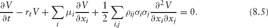
must be a martingale in the risk-neutral measure. Hence, applying Ito, we have
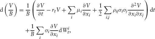
and so setting the drift to zero gives the PDE for V:
Next, we define the Arrow-Debreu price ψ(x′, t) as the present value of a derivative that pays off δ(xt − x′) at time t. This is related to the t−forward measure probability density of x, ϕ(x, t) by
as can be seen from the defining equations for ψ and ϕ:
The latter follows by noting that P(s, t) is the numeraire of the t−forward measure, ![]() , so
, so
![]()
To derive the forward PDE for ψ, we note that the left-hand side of equation (8.7) is independent of t. Differentiating both sides with respect to t, and using equation (8.5), gives
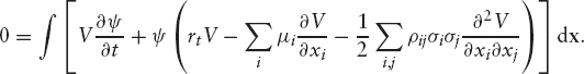
Integrating by parts, we get

These boundary terms depend on the specific problem. In all the cases we will discuss, μi and σi are well behaved everywhere, including infinity, so these boundary terms can be ignored. The above equation holds for all payoffs V(x, t), and so the only way in which it can hold generally is by setting
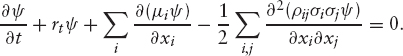
This is the PDE that we have been seeking for ψ.
We can remove the effect of deterministic interest rates or reduce the effect of jumps in the forward curve for stochastic interest rates by working with ϕ rather than ψ. If we let the forward short rate with maturity T, observed at t, be f(t, T), then
![]()
Using equation (8.6), we can show that ϕ obeys

The above equation demonstrates why it can be better in practice to work with ϕ rather than ψ. When interest rates are deterministic, rt − f(0, t) = 0, so the reaction term vanishes; when we use a Vasicek/Hull-White model for interest rates [61], [62], rt − f(0, t) is continuous, even if f(0, t) has discontinuities (which can happen if the yield curve is not interpolated smoothly). For more complicated rate models, such as Black-Karazinski ([63]), rt − f(0, t) will not be continuous, but its jumps will generally be much smaller than the ones in rt alone.
The initial conditions for ϕ or ψ can be found by taking the limit of the SDEs in equation (8.4) as t → 0. If the drift and volatility functions are bounded, then the equations reduce to
![]()
and so we can use an n-factor Gaussian as an initial condition at time δt. At time t = 0 the solution will be a delta function, so difficult to represent on a finite difference grid. An alternative approach is to rescale the coordinates near t = 0 so that the solution is a multifactor Gaussian is constant in the limit t → 0. We discuss this further in section 8.4.
Once we have ϕ(x, t), it is then easy to price any derivative with a European payoff at t by using equation (8.8). We can therefore price a whole series of European options with different strikes and maturities by propagating the solution for ϕ out to the latest maturity once. Note that this is only one example of a forward PDE. We show in section 8.3 that in a single-factor equity model (with no stochastic interest rates/hazard rates, etc.) we can derive a forward PDE for the call prices themselves as a function of their strikes and maturities.
8.3 PURE EQUITY CASE
In this section, we describe the equations governing the pure equity problem (by which we mean that there are no stochastic interest rates, credit, or volatility). We assume we have some stock S which pays a mixture of cash and proportional dividends as defined in section 1.1.1. Recall equation (1.6):
![]()
(![]() and At are defined in equations (1.7) and (1.8) of section 1.1.2.) We will use this to transform away the dividends and yield curve, leaving us with a martingale X, which we will assume follows the SDE
and At are defined in equations (1.7) and (1.8) of section 1.1.2.) We will use this to transform away the dividends and yield curve, leaving us with a martingale X, which we will assume follows the SDE
![]()
It will simplify the numerics (and in particular the boundary conditions that go into equation (8.9)) to work in log-space, so we define xt = ln(Xt/X0) and have
We will use σ(xt, t) as shorthand notation for σ(exp(xt),t). The meaning will always be clear from the context.
Using equation (8.10) from section 8.2, then provided σ is bounded as x → ±∞, we can ignore the boundary terms and get that
If we have computed ϕ(x, t) for some t, we can use it to price call options using equation (8.8):
![]()
where k is the strike transformed to log-space by
![]()
We also define a normalized call price
![]()
and get that
Obviously, we can price any European payoff using ϕ. However, if we are interested just in call prices (as is the case when calibrating a local volatility), we can instead write a PDE for c(k, t) and solve for the call prices directly. To do this, we start by differentiating equation (8.13) twice with respect to k, giving
![]()
This last equation allows us to convert from c to ϕ. Next, we differentiate c with respect to t, giving
![]()
where we have used equation (8.12) to eliminate ![]() Integrating by parts gives
Integrating by parts gives
By combining equations (8.14) and (8.17) we can eliminate ϕ(k, t), giving the desired PDE for c(k, t):
![]()
Rearranging this gives Dupire's formula in log-coordinates:
Now we have two ways to price European call options efficiently: solving the PDE for ϕ or solving the PDE for c. Note that the initial condition for c, c(k, 0) = (exp(k) − 1)+ is discontinuous in its first derivative in k, so for very short maturities we will have noise in the numerical solution. We can reduce this by taking smaller time steps and using a denser mesh near t = 0. Alternatively, we can solve for ϕ near t = 0, and switch to using the PDE for c at some larger t.
The initial condition for ϕ is even more pathological than the one for c, being a delta function. However, we can transform our x coordinate by ![]() where
where ![]() is some averaged implied volatility at time t, and work with ϕ′ (x′, t), where ϕ′ (x′, t)dx′ = ϕ(x, t)dx. The initial condition for ϕ′ is a Gaussian. Unfortunately, the coefficients of the transformed PDE become infinite as t → 0. To get around this, we could start the PDE from a small time δt, but in practice a second-order Crank-Nicholson scheme where the coefficients are evaluated halfway through a time step works even if started at t = 0.
is some averaged implied volatility at time t, and work with ϕ′ (x′, t), where ϕ′ (x′, t)dx′ = ϕ(x, t)dx. The initial condition for ϕ′ is a Gaussian. Unfortunately, the coefficients of the transformed PDE become infinite as t → 0. To get around this, we could start the PDE from a small time δt, but in practice a second-order Crank-Nicholson scheme where the coefficients are evaluated halfway through a time step works even if started at t = 0.
8.4 LOCAL VOLATILITY WITH STOCHASTIC INTEREST RATES
In this section, we derive the forward PDEs for a two-factor interest rate and equity model. As discussed in chapter 3, many short rate models can be expressed as follows:
where yt follows the Ornstein-Uhlenbeck process:
![]()
in the risk-neutral measure. The function ![]() is assumed to have been calibrated to fit the yield curve. If
is assumed to have been calibrated to fit the yield curve. If ![]() we have the extended Vasicek/Hull-White model, whereas if
we have the extended Vasicek/Hull-White model, whereas if ![]() we have the Black-Karasinski model. Of course, we could have written
we have the Black-Karasinski model. Of course, we could have written ![]() and this would have been equivalent mathematically. However, with the definition of equation (8.19), the function g is generally smoother (it is continuous in the Vasicek model, whereas the paths of rt may not be).
and this would have been equivalent mathematically. However, with the definition of equation (8.19), the function g is generally smoother (it is continuous in the Vasicek model, whereas the paths of rt may not be).
We have the stock price process in the risk-neutral measure:
![]()
The term νt encompasses all of the dividend/repo terms. To take these into account we change a variable, defining
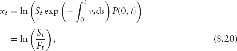
where Ft is the stock forward with maturity t. This new variable follows the process
Note that the deterministic interest rate case corresponds to gt(y) = 0, and equation (8.21) reduces to equation (8.11).
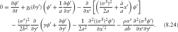
We have our SDEs for the two state variables, x and y, so we can apply equation (8.10) to get the PDE followed by the joint probability density ϕ(x, y, t):
In practice, this is a cumbersome PDE to solve: The initial condition at t = 0 is a two-dimensional delta function, and the distribution then spreads out as ![]() while the peak decreases as
while the peak decreases as ![]() Taking advantage of this information, we can rescale the x and y coordinates as
Taking advantage of this information, we can rescale the x and y coordinates as

where at and bt scale as ![]() as t → 0, and also rescale ϕ as
as t → 0, and also rescale ϕ as
![]()
Note that we have
![]()
so ϕ′ is just the probability density associated with the new coordinates x′ and y′.
We can use at and bt to make our PDE grid cover just the region where the probability density is significant. In the interest rate direction, we know that the marginal probability distribution is Gaussian with variance
![]()
and so we can define bt as the square root of this:

This makes y′ the number of standard deviations that the short rate is away from the mean.
The problem is more complicated in the equity direction, where we do not have a normal marginal probability distribution because of the volatility skew. However, we can compute the actual marginal probability distribution from call prices and use some feature of it to determine aT. One approach is to use the at-the-money implied volatility σatm and let
A better choice of at will allow us to distribute mesh points more efficiently in terms of speed of calculation for a given tolerance.
We get the following PDE for ϕ′:
Note that the coefficients diverge as t → 0. One approach is to move the initial condition to some small time δt; however, depending on the implementation of the PDE solver, this might not be necessary. The authors have obtained good results propagating from t = 0 with an ADI scheme where the coefficients are evaluated halfway through a time-step, hence avoiding the infinities at t = 0.
The initial condition for ϕ′ is a two-factor Gaussian; for small t we have
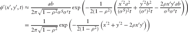
if we use a and b as in equations (8.23) and (8.4).
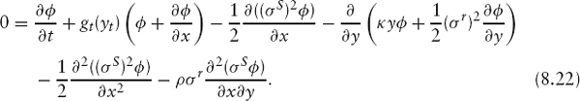
Figure 8.2 show the results of propagating equation (8.24) for 18 years using the volatility surface of the Nikkei index and a Hull-White model for the JPY interest rates with an instantaneous correlation of zero (the terminal distribution shown in the figure actually has some positive correlation from the effect of rate shifts on the growth rate of the index; see section 4.1). The long tail to the left of the distribution comes from the skew of the implied volatility surface; the in-the-money options have higher implied volatilities than out-of-the-money ones. The marginal distributions of x and y are shown in figure 8.3; note that in the interest-rate direction, we have just a Gaussian, as we are using a Hull-White model. In the equity direction, we have the same distribution we would get from solving the one-factor problem in section 8.3.
The coordinate rescalings are useful for the solution of the PDE but cumbersome when discussing the method, so we now return to working with ϕ. Inverting equation (8.20), the stock price is given by
![]()
FIGURE 8.2 The joint distribution ϕ(x, y) for the N225 and JPY after 18 years, with zero instantaneous correlation.
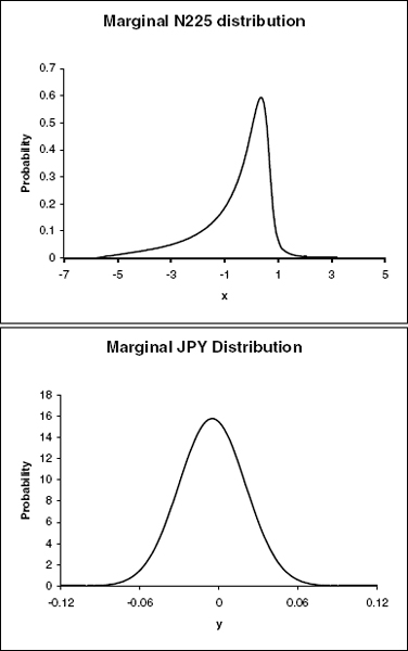
FIGURE 8.3 The marginal equity and interest rate distributions for N225 and JPY after 18 years.
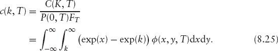
and so the price of a European call is given by
![]()
where
![]()
In an attempt to get a Dupire-like result, we can differentiate this expression with respect to k and T respectively. As in the previous section, in order to simplify the equations, we first write
Working in terms of c(k, T) rather than C(K, T), we don't have to worry about dividends or the initial yield curve. Differentiating with respect to T and using equation (8.22) gives
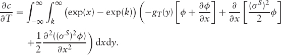
Integrating by parts a few times gives
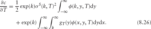
Differentiating equation (8.25) with respect to k gives

and so we can combine the last three equations to give
This is almost, but not quite, the Dupire-like result we want. Indeed, if we let gt(y) = 0 (which reduces the problem to the deterministic interest rate case), the above expression reduces to Dupire's formula. Unfortunately, there is no way to back out the second term on the right-hand side from just European option prices. However, if we have propagated ϕ up to time T, we can use the above expression to determine the local volatility between T and T + δT.
8.5 CALIBRATING THE LOCAL VOLATILITY
In the previous sections, we have shown how to use forward PDEs to price European options efficiently given a local volatility surface. It is then a standard inverse problem to find the local volatility surface that is consistent with an implied volatility surface. We can parameterize the local volatility in some way, then adjust the parameters until we correctly reprice a set of European options. Since the prices of European options with maturity T depend only on the local volatility surface at times t < T, we can bootstrap the calibration; that is, we can calibrate the surface up to some time Ti, then calibrate the surface from Ti to Ti+1, leaving the local volatility at t < Ti unchanged. We can also use ϕ(x, Ti), found in the calibration up to Ti, as a starting point for the calibration from Ti to Ti+1.
Depending on the amount of detail in the implied volatility surface we are trying to fit, we might want to parameterize the local volatility by tens or hundreds of parameters in any given time slice. The number of iterations that any root-finding algorithm is likely to need will grow accordingly. It can therefore become a very slow process to solve the inverse problem where the forward problem involves solving for ϕ with a one- or two- (or potentially higher) factor PDE solver. However, a better approach is available.
Assuming that we have evolved ϕ up to time t, we can write the call prices consistent with our local volatility surface as integrals over ϕ (see, for example, equation (8.25) for the two-factor version). We can then find a relationship between our local volatility σ(x, t) at this time and the rates of change of call prices with respect to maturity at fixed k. In one factor this is just equation (8.17) and in two factors it is equation (8.26). We can therefore express the call prices at time t + δt in terms of ϕ(t) and the local volatility between t and t + δt.
As an example, in the two-factor case we have
We want to find some function σ(x) that when applied between Ti and Ti+1, gives the minimum discrepancy between the model call prices c(k, Ti+1) and the market call prices cm(k, Ti+1). The above equation (and indeed the equivalent equation in the one-factor case) reduces to
![]()
where a and b are known at time T. We can iteratively guess the parameters of σ(x) until we minimize the above difference (in some norm). This is much faster than iterating the full problem, where c(k, Ti+1) is the result of an expensive PDE solution. Note that we could insist that the difference between the market and model call prices be zero, letting
![]()
The problems with doing this are that a might be negative (if the data are arbitrageable) and that at low/high strikes both a and b go to zero and the ratio of them cannot be computed with much confidence. A better approach is to minimize the difference between the model and the market call prices in some norm: ||c − cm||, plus some penalty function for nonsmooth σ(x) functions. We might want to minimize
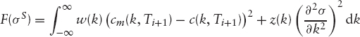
for some weight functions w(k) and z(k). Realistically, we would choose some discretised version of the above such as
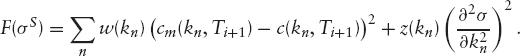
This function can be easily evaluated given a local volatility curve and does not involve expensive finite-difference computations, so we can back out the best local volatility curve using some least-squares fitting routine. It is also much safer to use a simple functional form in a minimization routine: the numerical noise in propagating with a PDE solver could easily confuse a minimization algorithm.
We can now use our local volatility with our slow finite-difference solver to propagate ϕ from Ti to Ti+1. Note that equation (8.28) is equivalent to using an explicit finite difference step to propagate from Ti to Ti+1, and the predicted call prices at time Ti+1 (and therefore the local volatility) are accurate only to O(δT), where δT = Ti+1 − Ti. However, while the call prices at Ti+1 from our local volatility surface might differ from the market call prices by O(δT), we know them to the same order of accuracy as our finite-difference solution. Any errors from the approximation will not accumulate but be corrected for on the next time step. The accuracy of our fit to the call prices is always O(δT), regardless of how many steps we are using to propagate up to time T providing our finite difference solver is accurate to at least O(δT2).
8.6 SPECIAL CASE: VASICEK PLUS A TERM STRUCTURE OF EQUITY VOLATILITIES
In this section, we show a quicker way to find a term structure of equity volatilities when the interest rates follow a Vasicek/Hull-White model and the stock has no implied volatility skew.
We have the risk-neutral dynamics
and
![]()
To remove the effects of the dividends, we define a new variable Xt by
![]()
which has the familiar dynamics
![]()
Xt corresponds to the strategy of reinvesting the dividends in the stock and so is tradable.
We want to find the dynamics of Xt in the T−forward measure, ![]() in which the zero-coupon bond P(t, T) is the numeraire; first, we must find the dynamics of P(t, T) under the risk-neutral measure
in which the zero-coupon bond P(t, T) is the numeraire; first, we must find the dynamics of P(t, T) under the risk-neutral measure ![]() . Integrating equation (8.29) gives
. Integrating equation (8.29) gives
![]()
The zero-coupon bond P(t, T) has value


where
![]()
Equation (8.32) gives us the volatility of the zero-coupon bond. We can find the drift using the fact that P(t, T) is tradable, so P(t, T)/Bt must be a ![]() −martingale and so we have
−martingale and so we have
![]()
Since Xt is tradable, Xt/P(t, T) will be a ![]() -martingale, so it follows that
-martingale, so it follows that
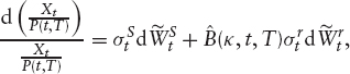
where ![]() are Brownian motions in
are Brownian motions in ![]() . It follows that under
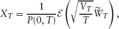
. It follows that under ![]() , XT is log-normally distributed with mean 1/P(0, T) (since X0 = 1) and variance
, XT is log-normally distributed with mean 1/P(0, T) (since X0 = 1) and variance
We can write
where ε is the Doléans-Dade exponential:
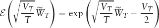
and so the stock price is given by
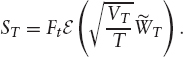
The price of a call with maturity T and strike K is
If we use the same assumptions that go into the definition of implied volatility (i.e., deterministic interest rates and a constant volatility), then we can identify
![]()
Substituting this into equation (8.33) gives the relationship between the implied volatility, σimp and the process volatilities, σS and σr:
To find σS from σimp and σr, we must invert the above expression. This can be done numerically by bootstrapping. Figure 8.4 shows the result for a constant implied volatility of σimp = 20%, with κ = 1% and σr = 2%, for a range of correlations. The larger the correlation, the more suppressed the local volatility becomes. Note that even with zero correlation, the process volatility is less than the implied volatility. Also note that we cannot fit a flat implied volatility beyond a certain maturity for each correlation.
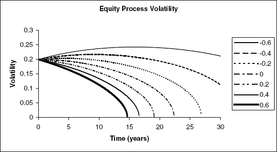
FIGURE 8.4 Equity process volatility for different correlations, with a fixed implied volatility of σimp = 20%, with κ = 1% and σr = 1%.