Chapter 4. Creating an Excel Prototyping Template
▪ Images and graphics
▪ Boxes and buttons
▪ Tab components
▪ Color key and palette
▪ Tips and tricks
▪ Table template
▪ Prototype starter worksheets
Templates
A template comprises worksheets in a special Excel workbook. The template contains user interface elements and useful information that you can use over and over as you build prototypes. By using a template as part of your prototyping practice, you have most of the prototyping building blocks you need available in one document.
The template facilitates collaboration with your team and stakeholders by enabling anyone who has the file to continue with the work that you started. Because the template is built from the canvas worksheet that you already set up, it has default specifications already integrated into the workbook. As you go through the process of building these template worksheets, you will gain a better understanding of how to use Excel for prototyping.
The Image Library
Nearly any prototype that you build will require some graphic elements. For example, you might need
You can store these graphics in an image library worksheet (Figure 4.1) for easy access so you can

▪ Reserve this worksheet for images that are not created in Excel.
▪ See the available images together on one worksheet.
▪ Group them in ways that make sense to you.
▪ Show them in context with each other; for example, the plus icon goes next to the minus icon.
▪ Copy many images at a time if needed.
What Graphics Should be Included in Your Image Library Worksheet?
There is no set number of images that you should include in your template. The image library is not intended to contain every graphic that you might ever need, but it is a place to keep the ones you think you will regularly use. In our experience at PeopleSoft and SAP, we found that only a small percentage of all the available graphics was needed to prototype most of the designs. Because the size of your workbook file could become large and cumbersome, take care not to accumulate too many graphics. Too many graphics could slow down your work and make your prototype less readily transportable. As you work on your project and find you need more graphics, you can always add them to the template as you evolve your designs.
Finding the Images You Need
Where can you find the images to put in your template? You have a few alternatives:
▪ Find appropriate graphics on another Website or application (paying appropriate attention to copyright issues).
▪ If you are working in a company that has a design or art department, it will often have an image library that you can use.
▪ Create them yourself.
▪ For some very simple graphics, Excel and other office applications have clip art that you can use.
When to Use Graphics Instead of Widgets Built in Excel
In subsequent chapters you will learn to build some widgets directly in Excel. How do you decide whether you should make your own each time in Excel or to save a graphic into your image library? Images that are specific to your site, such as logos, icons, or nonstandard buttons, would be good candidates for inclusion in the library. Parts of standard widgets that you will use all the time, such as the down arrow for a pull-down menu, are good to have available, and you can copy those directly from our templates.
Use the right level of fidelity in your prototypes. Not every prototype needs to be pixel-perfect. For example, is it important to have an exact copy of a Save button in a wireframe? Or is a generic Save button built with table cells in Excel good enough? See “Creating the boxes & buttons worksheet” below. The benefit of table cell buttons built in Excel is that you can change the text in the button at will, whereas you cannot change a static graphic button in Excel.
You will find a file of images on our Website for your use in building an image library: www.effectiveprototyping.com/ep_excel.
Save the file where you can access it easily while using this book.
To Create the Image Library
1 Open the Excel Canvas file that you created and saved earlier.
2 Right-click the Canvas worksheet tab and select Move or Copy (Figure 4.2).

3 In the Before sheet list in the Move or Copy dialog box, select (move to end) and select Create a copy; then click OK (Figure 4.3).

4 With the new tab selected, right-click and choose Rename.
5 With the tab text highlighted, type in Image Library (Figure 4.4).

Now that you have your Image Library worksheet, we'll show you how to add graphics to it.
To Add Graphics to the Template:
1 From the Draw toolbar, click Insert Picture From File (Figure 4.5). Alternatively, choose Insert > Picture and click From File.

2 Browse to where you saved the sample graphics file, exp.xls.
3 Select the graphic called exp_graphic1.gif; then click Insert. The inserted graphic will appear highlighted on the Image Library worksheet.
4 Do the same for graphics labeled 2–9.
The Boxes & Buttons Worksheet
This template worksheet includes different types of boxes and buttons that you will need as you design your interface (Figure 4.6). Although you might already have boxes or buttons that you copied on to your image library worksheet, these buttons are made from Excel table cells, borders, and text. You can change their size as well as the text so that they are much more flexible than static graphics.

The boxes (text entry fields, combo boxes, and so on) that are represented in Figure 4.1 were used in a Web application interface. By including this worksheet as part of your template, you will save yourself hours of work in the future.
Creating the Boxes & Buttons Worksheet
Start by opening your Excel template and right-clicking the Canvas tab to create a new worksheet the same way you created the Image Library. Name this worksheet boxes and buttons.
Boxes
Your first box is a combo box control that uses bordered table cells and a graphic from the Graphics Library (Figure 4.7, page 58).

To Create the Combo Box:
1 Using your cursor, select a horizontal area of cells.
2 With the cells highlighted, right-click and choose Format Cells (Figure 4.8, page 59).

3 Click the Border tab.
4 For this exercise you will change the default border color to a dark gray.
5 In the lower-right corner, click the down arrow next to Automatic under Color. A color palette will appear.
6 Select the middle gray by clicking it (Figure 4.9, page 60). All the line styles will now be this gray color.

7 Select the two-pixel line (Figure 4.10, page 61). In the center of the dialog box is a white box labeled Border with small tick marks. The tick marks represent the table cells that were highlighted on the worksheet.

8 Click in the upper-left part of the box with the arrow (Figure 4.11, page 62).

9 Then click the one-pixel line in the Style box.
10 Returning to the Border box, click the left and bottom sides of the box (Figure 4.12, page 63).

13 Click OK. After you deselect the table cells, you see a box that appears to be recessed, just like a normal input field (Figure 4.13, page 64).

14 Click your Image Library tab and find the gray box with the down arrow that you copied into the library previously. Right-click the graphic and choose Copy (Figure 4.14, page 64).
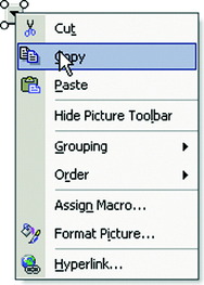
15 Return to the boxes and buttons worksheet and highlight the cell at the right end of the box that you just created. Paste the down arrow into the table cell (Figure 4.15, page 64).

You just created a combo box control (Figure 4.16, page 65).

To provide a range of boxes, repeat this process with different dimensions to create different variations and kinds of boxes (Figure 4.17, page 65).

Buttons
The buttons you create are also very simple in design. They might not look like the buttons you will end up using on your site, but they will express the idea of a button you'll need for a prototype.
When you built the input boxes, you created a widget that looked like it was inset. To create buttons, you will make a box that looks raised, as though you could click it.
To Create a Button:
2 Right-click the selected cells and choose Format Cells; then choose the dark teal color (Figure 4.18, page 66).

3 Choose the 2-pixel line style and click the bottom and right side of the Border box.
4 Return to the Color chooser and select a lighter teal color.
5 Still using the 2-pixel line, click the top and left sides of the Border box (Figure 4.19, page 67).

6 While still in the Format Cells dialog box, click the Patterns tab.
7 Select the lightest teal color (Figure 4.20, page 68), and then click OK.

8 Deselect the selected table cells and you will see the outcome of the button that you just created (Figure 4.21, page 69).

9 Highlight the center table cell of the five selected cells (Figure 4.22, page 69) and type in the word Save.

10 Click Center Text in the Formatting toolbar so that the text you entered is centered (Figure 4.23, page 69).
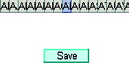
You have created a simple but effective Save button. Using these methods, you can create a wide variety of button styles and types to meet many of your user interface design needs (Figure 4.24, page 69).

Creating a worksheet of boxes and buttons in your template is an easy way to save time and effort when you are on a deadline and need to rapidly finish a prototype design. Remember, you don't have to make every variation of a button you will ever use. Once you are proficient at making these boxes and buttons, it is simply a matter of taking an existing box or button and modifying it to meet your needs.
The Tabs Worksheet
The tabs worksheet is another template worksheet that, if set up properly, can save you a great deal of prototyping time. As with the boxes & buttons worksheet, you can prebuild these interface features so that when you're in the middle of building a prototype you don't have to stop to figure out how to create tabs; you will already have them ready to use. In this exercise you will create a series of simple tabs, examples of which are shown in Figure 4.25 (page 70).

Follow the same procedure as in the previous sections to create a new worksheet named Tabs Straight.
To Create Straight Tabs:
2 With the cells still highlighted, right-click and choose Format Cells, then choose Patterns, select the dark teal color (Figure 4.26, page 71) and click OK.

3 In the same way that you inserted text in the button in the previous section, highlight the cell in the center of the tab. Type in Example Tab (Figure 4.27, page 71).

4 While you have the text highlighted in the Format Text toolbar, choose the Center Text icon. Then choose Bold and select white for the text color (Figure 4.28, page 72).

5 Skipping one table cell to the right of this tab, select the next nine table cells in the row. Follow the same procedure, except this time select a light gray color (Figure 4.29, page 72). The font style can be the default Arial regular with the default color black.

6 Highlight the light teal tab together with the empty cell to its left and copy these cells (Figure 4.30, page 72,).

7 Set the cursor directly to the right of the last gray cell. Using the Paste function (CTRL-V), paste in a new light teal tab. Repeat this two more times to finish the row of tabs (Figure 4.31, page 72).

In this design, you'll include a one-point black line under all the tabs extending across the entire tab area.
8 Select cells on the row of tabs, starting one cell to the left and extending 12 cells to the right of the last tab.
9 While the cells are selected, right-click and choose Format Cells and select the Border tab. Choose the one-point line style that has the Automatic color choice of black and click the bottom of the Border box (Figure 4.32, page 73).

You have created a complete row of tabs, with one of them highlighted (Figure 4.33, page 73).

To finish your tab worksheet, create a series of tab rows with different tabs highlighted. Use copy and paste to quickly create more tab rows.
To Create More Tabs:
2 Choose a cell that is two cells below the existing tab row; then paste a new row of tabs (Figure 4.34, page 73).

3 Repeat this three more times until you have created five stacked tab rows.
4 Now copy the highlight tab and paste it in a different sequential position on the remaining tab rows (Figure 4.35, page 73).

5 In each row, replace the extra highlighted tab with a gray tab (Figure 4.36, page 74).

Your tab row worksheet is now complete. You have a simple set of tabs that can easily be copied and pasted into a prototype design (Figure 4.37, page 74).

In making your own tabs worksheet, you can change the color or text to match your organization's house style. As you paste the tabs into a design, you can highlight the tab text and replace it with a context-appropriate name. If the tabs are too long or too short, you can add or subtract cells to adjust them.
Color Management
The Excel color palette lets you customize a palette for your specific needs and manage these palettes among your various prototypes. The default standard color palette has 50 colors (Figure 4.38, page 74).

You do not have to use only the colors that come with the default palette; you can create your own new custom colors.
To Create a New Color:
1 Click Tools > Options to open the Options dialog box.
2 Click the Color tab. The default palette opens.
3 Select a color that you want to customize; then click the Modify button.
You can choose a new color from a larger color palette or a palette that is made up of white, black, and gray tones. Once you've settled on a new color, you can click OK and the new color will replace the color you initially selected (Figure 4.39, page 75).


You see a palette with a much finer range of colors to choose from. The color value scale allows you to take whatever color you choose and move it up or down in the value range, making the color choice darker or lighter. If you want to make color selections that absolutely match specific colors, you can specify their color values in RGB.
5 When you are done creating or modifying colors, click OK.
Excel uses some default colors that you should not alter. Changing these colors might give you some unexpected results. If you change the blue that is used as the hyperlink color and the maroon (circled in figure) that is used for the visited hyperlink, Excel will use the colors that you changed them to. That might be what you want if the links in your design are not standard and you want them to be a different color by default; otherwise, they could cause unintended color changes (Figure 4.41, page 76).

The custom palette that you create will be saved in the workbook file. If you copy a prototype screen from this file into another workbook that is using the default palette or that uses a different custom palette, the colors in the copied workbook will change to those of the host workbook—which might cause some odd visual results.
The best solution is that everyone start with the same template. But you can copy and paste a color palette from one workbook to another. Use the Copy colors from drop-down list on the Tools > Options > Color tab. Select from the workbooks that are currently open, highlight the palette that you want to copy to your current document, and click OK (Figure 4.42).

The Color Key and Palette
The color key worksheet (Figure 4.43, page 78) serves as a color specification guide for anyone who is working on the prototype. You can create a custom palette, and all your collaborators will know exactly what colors should be used for what purpose.

The color key worksheet includes a screen capture of the custom color palette that you created, along with a numbered key that shows each of the different colors in use on a typical prototype screen. You can build this worksheet with any elements that you need to communicate your color palette. A high-fidelity prototype might include a detailed color worksheet, whereas a wireframe prototype that focuses on information architecture and is generally devoid of color might not need a color worksheet at all.
The Tips and Tricks Worksheet
Like the color palette worksheet, a tips and tricks worksheet (Figure 4.44, page 78) for your template will be primarily instructional. Tips and tricks would be a good place to pass on any information that is specific to building a particular design or to include instructions about your process. It's an ideal way to bring your project collaborators up to speed on how to best use this prototyping template.

The Table Template Worksheet
In building prototypes, you might find yourself repeatedly creating tables. The ability to create tables is one of Excel's best features for prototyping. You will be able to describe complex tables, build them very quickly, edit them, and copy and paste them into other worksheets.
You can create a table using patterns, text, and borders. You can
▪ Paste a table header onto a worksheet
▪ Change the text
▪ Paste column dividers
▪ Add text and widgets into the table
▪ Configure the spacing between rows
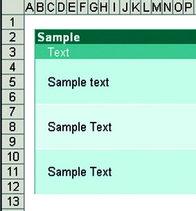
In these examples, the table is made up of a header, a subheader, and table rows. The rows in the table are built using alternating light and dark colors with a one-pixel white line between each row and column. Let's look at how to create the tables shown in Figure 4.45 and Figure 4.46 (page 80).


Creating the Table Template
Three rows are dedicated for each table row of one color. Look closely at the examples of the table in Figure 4.47. You will see that each table row is three worksheet rows deep, but two of the three rows are much shorter than the middle row. The middle row is for the content, whether it is text or a widget, such as a combo box. The reason for these added rows is twofold:

▪ For adequate spacing above and below your text and widgets
▪ To prevent distortion of your pasted graphics
The next part of the worksheet is made up of the vertical sections of the table. These are built similarly to the rows but have a vertical line and text that will be copied and pasted into the subheader row.
To Build a Table:
1 Create a new prototype screen from a canvas worksheet and call it Sample Table.
2 From the Tables worksheet in the provided sample template file, highlight and copy the header into the new worksheet along with all three rows (Figure 4.48).

4 In the subheader bar, type in Text.
You will notice that the white text style is part of the Table template (Figure 4.49, page 82).

5 Type into your sample table a line of text into each middle row. This will give you an idea of where to place your vertical divider lines (Figure 4.50, page 82).
6 From the Table Templates worksheet, highlight and copy a column (Figure 4.51, page 82) and paste it into the new table. Highlight one cell in the subheader to the right of where the text starts (Figure 4.52, page 83).


Now you can begin to see how the table will grow. You can fill in the rows and then add in new columns as needed. In this case type Name: in each row.
7 Next go to the boxes and buttons worksheet and copy a combo box. Return to the sample table and paste it next to Name:.
You don't have to return to the boxes and buttons worksheet each time. Just paste and reposition and paste again. Change the text in the column header to Names. Now you've completed another column (Figure 4.53).

Finish up the table by adding more sample data (Figure 4.54, page 84).

8 To adjust the table row heights, hold down the Control key while selecting each row that is above or below a content row, thus highlighting them all (Figure 4.55, page 84).

9 Right-click the left column and choose Row Height (Figure 4.56); specify 5 and click OK.

The results give you a nicely condensed box with spacing around the content.
Finish the table by highlighting the whole table and adding a border by using the Format menu (Figure 4.57).

Modifying the Table
Nothing is ever finished in a prototype. So how will you iterate with tables?
▪ If you just need to change the content, highlight the text and replace it with new text.
▪ If the column is too narrow, copy a portion of the column and paste it to the right or left to increase the column width.
▪ If your changes are complicated, return the table to its original state with three-deep rows per table row. Highlight all the rows from the far left column, choose Row Height, and return the rows to the original height of 13 (Figure 4.58, page 86).

If you get comfortable with using the Table Template worksheet, you can get the most out of the speed, flexibility, and power of Excel prototyping.
The Starter Worksheet
Another useful template worksheet is a starter worksheet. The example in Figure 4.59 is a starter worksheet from the sample Arnosoft site. Notice the global elements, such as the top navigation bar and logo. The layout of the worksheet follows a design that might be found on many Arnosoft prototype screens. By including a worksheet in your template, which already has many of the global elements, you can use it to start new prototypes without having to start from scratch every time. You can save time by having everything placed correctly with many of the widgets you think you'll need.

The contents of a starter worksheet will depend on the design that you are prototyping. You might have more than one starter worksheet, depending on your designs. Don't try to anticipate every starter worksheet that you might need—you don't want to fill up your template with unnecessary worksheets.
You can also backfill as needed. If you start a new design and think that you're going to use that design a lot, copy and save it as a starter worksheet that you can reuse later.
Conclusion
As you worked through the exercises in this chapter, you created your own template. From the canvas, the fundamental starting point for prototyping in Excel, you created the various template worksheets. In the coming chapters we will discuss how you can use this template to create different types of prototypes.
..................Content has been hidden....................
You can't read the all page of ebook, please click here login for view all page.