5 Elliptic curves

Johann Carl Friedrich Gauss (1777–1855) showed that the complex numbers ℂ can be identified with the plane ℝ × ℝ. By contracting the infinitely far border of this plane to a single point, we obtain the surface of a sphere. The extra point in the drawing corresponds to the North Pole and the real numbers together with this point appear as a circle on the sphere.

The typical shape of an elliptic curve over ℂ is more complicated and it emerges when we consider a grid. In the simplest case, this is the additive subgroup L = ℤ+ iℤ. For the grid L, we can form the quotient group ℂ/L. We can visualize this group as a three-dimensional image similar to the surface of a sphere. However, ℂ/L does not give a sphere but a torus, that is, the surface of a donut. We start with the unit square [0, 1] × [0, 1] inside ℝ×ℝ. Then, the four edges of [0, 1] × [0, 1] belong to the grid L (when identifying ℝ×ℝ with ℂ); and we obtain ℂ/L by glueing together the top and the bottom edge as well as the left and the right edge. This results in a torus as a visualization of ℂ/L. In ℂ/L, seen as an additive group, there are exactly four elements of order at most 2. In the unit square [0, 1] × [0, 1], they correspond to the points (0, 0), (0, 1/2), (1/2, 0), and (1/2, 1/2). Thus, the Klein four-group ℤ/2ℤ×ℤ/2ℤappears as a subgroup of ℂ/L.

Consider a cubic equation of type Y2 = X 3+AX+B with constants A and B and two variables X and Y over the complex numbers ℂ; and let E = {(a, b) ∈ ℂ×ℂ| b2 = a3 + Aa +B } be its set of solutions. If the roots of the polynomial X3+AX+B are all different, then E is a smooth surface of (real) dimension 2 inside the space ℂ×ℂof dimension 4. The set E can naturally be identified with the surface of a torus; as in the step from a plane to a sphere, one has to add some extra “point at infinity.” The connection between E and the surface of a torus is given by the following parametrization: there exist w1, w2 ∈ ℂ {0} with and a total function f : ℂ → ℂ ∪ {∞} with f(z) = f(z + w) for all w in the grid L = {mw1 + nw2 |m, n ∈ ℤ} such that

As a partial mapping from ℂtoℂ, the function f is meromorphic and f' is its derivative; we set f' (z) = ∞whenever f' (z) is undefined over ℂ. The parametrization has the additional property that the mapping ℂ/L → E ∪ {(∞, ∞)} with z ↦ (f(z), f' (z)) is bijective. This allows us to identify E ∪ {(∞, ∞)} with the torus ℂ/L. A meromorphic function f with f(z) = f(z + w) for all w ∈ L is called elliptic; and the above connection coins the term elliptic curve. For more details on parametrizations of elliptic curves, we refer to the existing literature and textbooks such as [57] or [90].

The real solutions of Y2 = X3 + AX + B can be obtained as the intersection of a plane and the torus defined by E. For instance, taking the intersection of the torus with the equatorial plane, we obtain two circles, one positioned inside the other. If we cut the outer circle and pull the endpoints to infinity, then the standard image of an elliptic curve over the real numbers emerges (see the second plot in Figure 5.1), and the points on this curve still satisfy the cubic equation. We can imagine that, in this case, the point (∞, ∞) from the torus has become an infinitely distant point, called the point at infinity.

The three plots in Figure 5.1 show the elliptic curves (over ℝ) given by the equations Y2 = X3 − X + B with B ∈ {−1, 0, 1}. The third one, for example, shows the set of points

Fig. 5.1. Elliptic curves over ℝ.

We call such a set of points a curve. If (a, b) is a point on the curve, then (a, −b) is another one. The picture does not really look like an ellipse and, in fact, the connection between ellipses and elliptic curves can only be understood via a detour to elliptic functions.

Due to our focus on discrete methods, elliptic curves over finite fields are of particular interest. To this end, we start with an algebraic equation Y2 = X3 + AX + B with coefficients in ℤ and investigate the points satisfying this equation modulo some prime p, that is,

where p denotes the finite field ℤ/pℤ. Figure 5.2 gives two examples of such “curves” for p = 101. There are some hidden lines and circular structures, but the exact scheme looks rather random. This “regular chaos” makes elliptic curves of significant interest for cryptographic applications.

Fig. 5.2. Elliptic curves over ℤ/101ℤ.

In the distant future, the Rivest–Shamir–Adleman (RSA) algorithm could be broken, while cryptography using elliptic curves might remain secure. It is widely believed that techniques such as the quadratic sieve (Section 3.6.3) or the index calculus method (Section 3.7.4) cannot be efficiently adapted to elliptic curves; this approves the use of elliptic curves in cryptography and it is the main reason for smaller key sizes in elliptic curve cryptosystems. The position of the points follows a precise geometric structure, thereby forming an Abelian group. A computer is able to perform computations in this group’s structure very efficiently. The fascination of elliptic curves has influenced whole generations of mathematicians. The study of such curves lead Andrew Wiles (born 1953) and Richard Taylor (born 1962) to the proof of Fermat’s Last Theorem, which states that, for every integer n ≥ 3, the equation Xn + Yn = Z n has no positive integer solution.

In the following, let K denote a field and k an algebraically closed field containing K. Thus, k is always infinite; it is a field extension of K in which each polynomial splits into linear factors. For K = ℚ or K = ℝ, we choose k = ℂ. For K = p, we content ourselves with the knowledge that an algebraic closure exists and that it is infinite. We do not treat the subject in full generality: fields of characteristic 2 are omitted completely, and for characteristic 3, we only consider curves in Weierstrass normal form (Karl Theodor Wilhelm Weierstrass, 1815–1897). A general elliptic curve is defined by an equation of the form

for constants A, B, C, D, and E. The equation is in Weierstrass normal form if C = D = E = 0. If the characteristic is neither 2 nor 3, then, by affine transformations, every elliptic curve is equivalent to one in Weierstrass normal form; see Exercise 5.1.

We choose coefficients A, B ∈ K and consider the polynomial s(X) = X3 +AX+B = (X − a1)(X − a2)(X − a3). We are only interested in the (generic) case where the three roots a1, a2, a3 ∈ k are pairwise distinct. This is equivalent to 4A3 + 27B2 ≠ 0; see Exercise 5.2. The polynomial s(X) leads us to an equation with two variables

The solutions of this equation can be interpreted as a curve in K × K. We call the set

an elliptic curve over K. In particular, E (K) is a subset of E (k). As we have seen earlier, it is natural to add a so-called point at infinity, denoted by O. By abuse of notation, we also call

an elliptic curve. In projective coordinates, the point at infinity would belong to the curve in a natural way from the very beginning.

Unlike E (K), the curve E (k) always contains infinitely many points: since k is algebraically closed, we can always extract square roots. In particular, for each of the infinitely many a ∈ k there exists b ∈ k with (a, b) ∈ E(k).

For a point P = (a, b) ∈ k×k,wedefine and Thus, besides, exactly the three points Pi = (ai , 0) in Ẽ(k) satisfy As we will see later, these four points form a Klein four-group with as the neutral element. If the polynomial s(X) already splits into linear factors over K, then the points Pi are in E (K).

Formula (5.1), in a way, provides a connection between chance and necessity6. Suppose for every a ∈ q, we independently and uniformly at random chose c ∈ q and counted the pairs (a, b), (a, −b) if and only if c = b2 is a square. Then, wewould expect q pairswith a deviation of about One can think of c as a randomized equivalent of s(a). By Hasse’s theorem, this probabilistic behavior coincides rather precisely with the actual bounds.

5.1 Group law

The interest in elliptic curves in the context of cryptography or number theoretic algorithms is based upon a binary operation + on E ̃(K) such that (Ẽ(K), +, ) forms an Abelian group.We present a geometric approach, which uses lines and their intersection with E ̃(K) as an approach to define the addition. It turns out to be quite obvious that +maps two points of Ẽ(K) to a point on E ̃(K), that is the neutral element, every point has an inverse, and + is commutative. The only unobvious property is associativity, which is surprisingly difficult to prove. We give a complete and self-contained proof of associativity in Sections 5.1.2 and 5.1.3.

5.1.1 Lines

A line in k × k is a set of points L that can either be described by the equation X = a or by Y = μX+ν. In the first case, we speak of a vertical. We imagine the point at infinity O lying on every vertical but on no other line.

We investigate the intersection of lines with points on an elliptic curve E (k) given by Y2 = s(X) with s(X) = X3 + AX + B. If L is a vertical given by X = a, then the points P = (a, b) and are in the intersection L ∩ E(k) whenever b2 = a3 + Aa + B. For b = 0, we have and the point is counted twice. Together with the point at infinity , this gives exactly three points in the intersection of E ̃(k) and the vertical.

If L is described by the equation Y = μX + ν and if P = (a, b) belongs to the intersection of L and E (k), then a is a root of the following polynomial:

This polynomial of degree 3 over k has exactly three (not necessarily distinct) roots, and each root uniquely defines an associated Y-coordinate via the linear equation. If we write t(X) = (X − x1)(X − x2)(X − x3), then a ∈ {x1, x2, x3} and, by comparing the coefficients of X2, we obtain x1 + x2 + x3 = μ2. Let yi = μxi + ν for i ∈ {1, 2, 3}. Then, we obtain

If we know the two points (x1, y1) and (x2, y2), then we can determine the third point (x3, y3) using the following formulas:

We find the parameter ν by

To determine the parameter μ, we have to distinguish between the cases x1 ≠ x2 and x1 = x2. Assume that x1 ≠ x2. Then, μ can be computed as

Otherwise, if x1 = x2, then x1 is a double root of t(X), and we have

We have y1 ≠0 because otherwise s'(x1) = 0, that is, x1 would also be a double root of s(X), a case which we have excluded from our considerations. Together with the fact that 2 ≠ 0 in k, this yields 12

The value μ is the slope of the tangent of the elliptic curve at the point (x1, y1).

Many computations can be performed in the field K without having to consider the algebraic closure k. Let x1, A, B, μ, ν ∈ K and as given earlier t(X) = s(X) − (μX + ν)2 = (X − x1)(X − x2)(X − x3). Then, x2 ∈ K if and only if x3 ∈ K. If x2 is in K, then L ∩ E(k) = {(xi , yi) | i = 1, 2, 3} ⊆ E(K). Thus, if two points of a line belong to Ẽ(K), then the third point is in E ̃(K), too. This leads to the crucial idea of how to obtain the commutative group structure on the set E ̃(K). We let the point at infinity O be the neutral element, and the sum of any three points of E ̃(K) (with multiplicities) lying on a common line is defined to be zero.

We make this explicit by giving formulas for the group operation. Several cases need to be distinguished. For all P ∈ E ̃(K), we define P + = + P = P. The sum of two points P = (x1, y1) and Q = (x2, y2) of E(K) is computed as follows:

(a)If x1 ≠ x2, we draw a line through P and Q. This means we compute and x3 = μ2 − x2 − x1 and finally y3 = y1 + μ(x3 − x1). We let and

(b)If x1 = x2 and y1 ≠ −y2, then y1 = y2 ≠ 0 and P = Q. We determine the tangent slope and x3 = μ2 − 2x1 as well as y3 = y1 + μ(x3 − x1). The third point on the line through P and Q is R = (x3, y3). To achieve P + Q + R = , we define

(c)Finally, if x1 = x2 and y1 = −y2, then P and Q are on a vertical, and the third point on this line is Therefore, we define

Theorem 5.1. The aforementioned operation on E ̃(K) defines the structure of an Abelian group with as its neutral element.

Proof: We have already seen that P + Q ∈ E ̃(K) for P, Q ∈ E ̃(K). From the rules given earlier it follows that

□

The only condition which is not clear and, in fact, difficult to show, is the associative law

(P + Q) + R = P + (Q + R)

In order to show associativity, we take a detour via polynomials. The presentation of this proof is the subject of the following two sections.

5.1.2 Polynomials over elliptic curves

We define and investigate polynomials over E (k). As given earlier, let s(X) = X3 + AX + B. Let a1, a2, a3 ∈ k be the roots of s(X); they are assumed to be pairwise different. The polynomial ring in two variables X and Y is denoted by k[X, Y]. Each polynomial f(X, Y) ∈ k[X, Y] can be evaluated at (a, b) ∈ k × k to obtain f(a, b). We restrict

ourselves to the evaluation at points of the elliptic curve. At these points, the evaluation of f(X, Y) ∈ k[X, Y] coincides with the evaluation of

for each polynomial h(X, Y) ∈ k[X, Y]. Thus, in the ring k[X, Y] we can introduce an equation Y2 = s(X) and consider the quotient ring

where 〈Y2 = s(X)〉 is the ideal generated by Y2 − s(X). We call k[x, y] the polynomial ring over E (k). The element x ∈ k[x, y] is the residue class of X modulo 〈Y2 = s(X)〉 and, similarly, y is the residue class of Y. For a polynomial f ∈ k[x, y] and a point P = (a, b) ∈ E (k), the value f(P) = f(a, b) ∈ k is well defined, since all polynomials g in the residue class of f satisfy g(P) = f(P) for all P ∈ E(k). In the following, we show that the ring k[x, y] behaves very similarly to the usual polynomial ring. To this end, we introduce the norm of a polynomial, which allows us to use our knowledge about polynomials in one variable. Using the norm, we introduce a notion of degree that satisfies the degree formula. The usual notion of a degree cannot be used here since, for example, y2 = s(x) would have both degree 2 and degree 3. Then, we show that, for points on the elliptic curve, the order of a root can be defined in a reasonable manner. It is not entirely obvious how this can be achieved since, for instance, the point (a1, 0) of the elliptic curve is a root of the polynomial x + y − a1, but neither x − a1 nor y can be factored out. By k[x], we denote the image of the polynomial ring k[X] in k[x, y]. It is clear that k[X] can be identified with k[x]. Note, however, that (y3 − y2)(y + 1) is in k[x] while neither y3 − y2 nor y + 1 is in k[x].

Every polynomial f ∈ k[x, y] can be written as f = υ(x) + y ⋅ w(x) for υ(x), w(x) ∈ k[x]: Suppose that f = Σi≥0 fi(x)yi for fi(x) ∈ k[x]. Then

and we can set υ(x) = Σi≥0 f2i(x)si (x) and w(x) =Σi≥0 f2i+1(x)si (x).

Lemma 5.2. If f ∈ k[x, y] is a polynomial with f ≠ 0, then it has only a finite number of roots in E(k).

Proof: Let f = υ(x) + y ⋅ w(x). We reduce the problem to a polynomial with only one variable. Consider

If f(P) = 0 for infinitely many P ∈ E (k), then the polynomial g has infinitely many roots in k. Thus, it is the zero polynomial. Since the degrees in x of w2(x) and υ2(x),respectively, are even (or−∞) but the degree of s(x) is 3, it follows that υ(x) = w(x) = 0 and thus f = 0.

□

The lemma implies uniqueness of the representation f = υ(x) + yw(x). To see this, let υ(x)+yw(x) = υ̃(x)+yw̃ (x) and consider g = υ(x)−υ̃(x)+y(w(x)−w̃ (x)). Then, g(P) = 0 for all P ∈ E (k), and thus, from Lemma 5.2 we obtain υ(x) = υ̃(x) and w(x) = w̃ (x).

For f = υ(x) + yw(x) ∈ k[x, y], we define by Since the representation f = υ(x) + yw(x) is unique, is well defined. Implicitly, was already used in the proof given earlier, even though we did not know (and did not use) that f it is well defined. We can now formally define the norm of f :

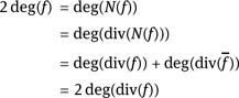
Thus, the norm N (f) is a polynomial in k[x]. In particular, the norm of x is x2 and the norm of y is −s(x). One can easily check that N(f ⋅ g) = N(f) ⋅ N(g). For f ∈ k[x] let degx(f) be the degree of f as a polynomial in k[X]. Then, we have

This holds because the degree of υ2(x) is even (or −∞) but the degree of s(x)w2(x) is odd (or −∞). Moreover, we note that N (f) = 0 implies f = 0. We define the degree of f ∈ k[x, y] by

Note that deg(f) can never be 1, whereas all other values −∞, 0, 2, 3, . . . are in the image of deg. In the following, we will see that this is a key idea for understanding elliptic curves. The degree mapping factors are as follows:

These mappings are monoid homomorphisms, where the operations in k[x, y] and k[x] are multiplicative while in {−∞} ∪ ℕ it is additive. Let us keep in mind that deg(f) ≠ 1 and deg(fg) = deg(f) + deg(g) for all f, g ∈ k[x, y].

Suppose that fg = 0 in k[x, y]. Then, N(f)N(g) = 0 in k[x] and therefore N(f) = 0 or N (g) = 0. This implies f = 0 or g = 0, thereby showing that k[x, y] is an integral domain, that is, the zero polynomial 0 is the only zero divisor.

Next, we want to define the order ordP(f) of a polynomial f ∈ k[x, y] at a point P ∈ E(k). Remember that, over an algebraically closed field k, every polynomial f ∈ k[X] can be split into linear factors

where di is the order (or multiplicity) of the root xi ∈ k and For polynomials f ∈ k[x, y], the situation is quite similar.

Theorem 5.3. Let f ∈ k[x, y] with f ≠ 0 and P = (a, b) ∈ E(k). For exactly one d ∈ ℕ there exist g, h ∈ k[x, y] such that g(P) ≠ 0 ≠ h(P) and

where a1, a2, a3 are the roots of s(X).

Proof: First, we show the uniqueness of d for a ∉ {a1, a2, a3}. Consider fg = (x − a)dh and f g̃ = (x−a)eh̃ for d > e ≥ 0.We obtain (x−a)dg̃h = fgg ̃ = (x−a)eh̃g and therefore

Since (x − a)e is not the zero polynomial, we obtain (x − a)d−eg̃h = h̃g. Using d > e we see that ((x − a)d−eg̃h)(P) = 0 and thus (h̃g)(P) = h̃(P)g(P) = 0. This shows that g(P) = 0 or h̃(P) = 0. Hence, for every a, there is at most one d satisfying fg = (x−a)dh and g(P) ≠ 0 ≠ h(P).

Next, we show the uniqueness of the exponent d for a ∈ {a1, a2, a3}. Note that in this situation, we have b = 0. Let fg = ydh and f g̃ = yeh̃ for d > e ≥ 0. As before, we obtain

Since ye is nonzero, this yields yd−eg̃h = h̃g. Now, d > e implies yd−eg̃h(P) = 0 and thus h̃(P)g(P) = 0. Therefore, g(P) = 0 or h̃(P) = 0.

We now prove the existence of d. By Corollary 1.47, there exists an integer e ≥ 0 and polynomials υ, w ∈ k[x] with

and υ(a) ≠ 0 or w(a) ≠ 0. First, consider the case a ∉ {a1, a2, a3} and b ≠ 0. If υ(a) + bw(a) ≠ 0, we can choose d = e, g = 1 and h = υ(x) + yw(x). If υ(a) + bw(a) = 0, then υ(a) − bw(a) ≠ 0 has to hold because otherwise 2υ(a) = 0 = 2bw(a) in contradiction to υ(a) ≠ 0 or w(a) ≠ 0. Thus, the polynomial g = υ(x) − yw(x) satisfies g(P) ≠ 0 and fg = (x − a)eN(g). The polynomial (x − a)eN(g) is in k[x] and can thus be written as (x − a)dh(x) with h(a) = h(P) ≠ 0.

For the other case, without loss of generality we may assume that a = a1 and b = 0. Then

For υ(a) ≠ 0 we can choose d = 2e and g = (x − a2)e(x − a3)e and h = υ(x) + yw(x) since b = 0 ensures h(P) = υ(a). In the case of υ(a) = 0, we have υ(x) = (x − a)cυ̃(x) for c > 0 and υ̃(a) ≠ 0. This yields

with w̃ (x) = (x−a2)c(x−a3)cw(x). Note that w̃ (a) ≠ 0. If we let h = w̃ (x)+ysc−1(x)υ̃(x), then also h(P) = w̃ (a) ≠ 0 because b = 0. Then

and we have reached our goal with d = 2e + 1.

□

For a polynomial f ≠ 0 and a point P ∈ E (k) let d ∈ ℕ be defined as in Theorem 5.3. We call d the order of f at P and write d = ordP(f). Note that f(P) = 0 if and only if ordP(f) > 0. If ordP(f) > 0, we also speak of the multiplicity of the root P. An important property of the order follows directly from the uniqueness in Theorem 5.3:

for all f, g ∈ k[x, y] and P ∈ E(k).

Theorem 5.4. Let f, h ∈ k[x, y] with f ≠ 0 ≠ h and ordP(f) ≤ ordP(h) for all P ∈ E(k). Then, there is a polynomial g ∈ k[x, y] satisfying fg = h.

Proof: It suffices to show the existence of g ∈ k[x, y] with since then and thus fg = h. Because of for all points P, by replacing f by we may thus assume that f ∈ k[x]. We use induction on the degree of f. If degx(f) = 0, then f ∈ k is a constant and g = f −1h satisfies the requirements of the theorem. For degx(f) = 1, it is sufficient to consider the normalized case f = x − a. Let h = υ(x) + yw(x) and let P = (a, b) be a point on the curve. From we obtain ordP(h) ≥ 1 and Thus υ(a) + bw(a) = 0 = υ(a) − bw(a). For b ≠ 0 this yields υ(a) = w(a) = 0 and, hence, h contains a factor x − a. The remaining case is b = 0, υ(a) = 0 and w(a) ≠ 0. We may assume that a = a1. Since (x − a)(x − a2)(x − a3) = s(x) = y2, we have ordP(x − a) = 2. On the other hand, ordP(h) = 1 because

□

Here, w̃ (x) = (x − a2)(x − a3)w(x), and υ̃(x) is determined by υ(x) = (x − a)υ̃(x). This contradicts ordP(x − a) ≤ ordP(h). Therefore, the situation b = 0, υ(a) = 0 and w(a) ≠ 0 cannot occur for degx(f) = 1.

Now let degx(f) > 1. Then, f can be written as f = f1f2, where both degx(f1) and degx(f2) are smaller than degx(f). We can apply the induction hypothesis to f1 and h. This yields the existence of g1 ∈ k[x, y] with f1 ⋅ g1 = h. Now, ordP(f2)≤ ordP(g1) for all P ∈ E(k). Again, by induction there exists g2 ∈ k[x, y] with f2g2 = g1. Thus, we obtain fg2 = f1f2g2 = f1g1 = h.

5.1.3 Divisors

A divisor (with nonnegative coefficients) in this context is a formal sum where n P ∈ ℕfor all P and n P = 0 for almost all P. Therefore, the sum is finite. Divisors can be added:

Note that the addition of divisors is associative. The empty sum with n P = 0 for all P ∈ E (k) is the neutral element. The degree of a divisor D = ΣP∈nP n PP is given by

Obviously, deg(D1 + D2) = deg(D1) + deg(D2). By Lemma 5.2, every polynomial f ∈ k[x, y] defines a unique divisor div(f) by

Since ordP(f ⋅ g) = ordP(f) + ordP(g), it follows that div(f ⋅ g) = div(f) + div(g). Divisors of type div(f) are called principal divisors. Let us first determine the principal divisor of f = x − a. Let P = (a, b). If a ∈ {a1, a2, a3}, say a = a1, then we have (x − a)(x − a2)(x − a3) = s(x) = y2 and hence ordP(x − a) = 2; this yields div(x − a) = 2P. For a ∉ {a1, a2, a3}, we have and So regardless of a, we always obtain div(x − a) = P + P.

In the next step let f = f(x) ∈ k[x]. Then, with If we choose elements yi ∈ k such that Pi = (xi , yi)∈ E(k), then the principal divisor of f is

Then for f ∈ k[x], we obtain the formula

For a divisor D = ΣP∈E(k) nPP we further define Obviously, deg(D) = Now let f ∈ k[x, y], then It follows that and therefore We obtain

This yields

Therefore, a principal divisor can never have degree 1. Since for P = (a, b) ∈ E (k) the divisor is a principal divisor, all divisors of type are principal divisors.

Let us examine the principal divisors of a linear polynomial f = μx + ν + γy for μ, ν, γ ∈ k. The case γ = 0 has already been treated earlier. So, without loss of generality let γ = −1. The principal divisor can be obtained from the three points in the intersection of the line L = {(x, y) ∈ k × k | y = μx + ν } and the elliptic curve. The corresponding formulas can be found in Section 5.1.1.

5.1.4 Picard group

In the following, all computations are performed modulo principal divisors. Formally, we define an equivalence relation by C ∼ D if there exist polynomials f, g ∈ k[x, y] such that C +div(f) = D +div(g). Then [D], as usual, denotes the equivalence class of D. If C1 ∼ D1 and C2 ∼ D2, then also C1+C2 ∼ D1+D2. Thus, the set of equivalence classes is a commutative monoid with respect to the operation [C]+[D] = [C+D]. All principal divisors are in the same class, which is the neutral element 0. This monoid is in fact a group because is a principal divisor, that is, and hence The group consisting of these classes is called the Picard group (Charles Émile Picard, 1856–1941) and it is denoted by Pic0(E(k)). We show that the Picard group Pic0(E(k)) can be identified with Ẽ(k).