Chapter 3: Key Features and Use Cases – Your Distributed Database Essentials

If you have completed the previous chapter, then you will have already acquired an understanding of how Apache ShardingSphere is built, its kernel, and its architecture.

You may also remember how the previous chapter introduced some features that are located in the third layer (L3) of ShardingSphere's architecture. This chapter will introduce you to the most important features of Apache ShardingSphere: the features that will allow you to create a distributed database and perform data sharding – including how they are integrated into its architecture and how they work.

After completing this chapter, you will have expanded your knowledge of the architecture that you gathered in the previous chapter, not only with new knowledge about each specific feature but also the key use cases for each feature.

As you may recall, in Chapter 1, The Evolution of DBMSs, DBAs, and the Role of Apache ShardingSphere, we introduced you to the main pain points that database professionals, as well as businesses at large, are facing as a result of digital transformation and the app economy. Reading this chapter will allow you to connect each feature and its respective use case with a corresponding real industry pain point.

After reading this chapter, you will have mastered the features of Apache ShardingSphere that are necessary for a distributed database, their use cases, and the pain points that they address.

These features include read/write splitting, high availability, observability, and data encryption. The common themes that tie these features together are performance and security; implementing them will allow you to improve your system's performance and security.

In this chapter, we will cover the following topics:

• Distributed database solutions
• Understanding data sharding
• Understanding SQL optimization
• Overview and characteristics of distributed transactions
• An introduction to elastic scaling
• Read/write splitting

Distributed database solutions

In the context of the current internet era, business data is growing at a very high pace. Faced with storage and access to massive amounts of data, the traditional relational database solution of single-node storage is experiencing significant challenges. It is difficult to meet massive data in terms of its performance, availability, operation, and maintenance cost:

• Performance: Relational databases mostly use B+ tree indexes. When the amount of data is too large, the increase in the index depth will increase the amount of disk access I/O, resulting in the decline of query performance.
• Availability: As application services are stateless, they can realize low-cost local capacity expansion making the database become the bottleneck of the whole system.It has become increasingly difficult for traditional single data nodes or primary-secondary architectures to bear the pressure of the whole system. For these reasons, databases' availability has become increasingly important, to the point of becoming any given system's key.
• Operation and maintenance costs: When the amount of data in the database instance increases to a certain level, the operation and maintenance costs will greatly increase. The cost in terms of time lost for data backup and recovery will eventually grow exponentially, and in a way that is directly proportional to the amount of data being managed. In some cases, when relational databases cannot meet the storage and access requirements of massive data, some users store data in the original NoSQL that supports distribution. However, NoSQL has incompatibility problems with SQL and imperfect support for transactions, so it cannot completely replace the relational database – and the core position of the relational database is still unshakable.

Facing this rapid expansion in the amounts of data to be stored and managed, the common industry practice is to use the data fragmentation scheme to keep relational databases' data volume of each table below the threshold by splitting the data, to meet the storage and access requirements of massive data.

The key method to achieve this is via data sharding, which is not to be confused with data partitioning. In the next section, we will introduce you to data sharding, why sharding might be the answer to your data storage issues, and how Apache ShardingSphere supports and implements this technology.

Understanding data sharding

Data sharding refers to splitting the data in a single database into multiple databases or tables according to a certain dimension, to improve performance and availability.

Data sharding is not to be confused with data partitioning, which is about dividing the data into sub-groups while keeping it stored in a single database. Many other opinions and ideas are floating around in academia and on the internet about this, but rest assured that the number of databases where the data is stored represents the main difference that you should be aware of when distinguishing between sharding and partitioning.

According to the granularity of data sharding, we can divide data sharding into two common forms – database shards and table shards:

• Database shards are partitions of data in a database, with each shard being stored in a different database instance.
• Table shards are the smaller pieces that used to be part of a single table and are now spread across multiple databases.

Additionally, database shards can efficiently disperse the number of visits to a single point of the database and alleviate the pressure on the database. Although table shards cannot alleviate database pressure, they can convert distributed transactions into local transactions, avoiding the complexity that's brought by distributed transactions.

According to the data sharding methodology, we can divide data sharding into vertical sharding and horizontal sharding. Let's dive deeper into the characteristics of both types of sharding.

Understanding vertical sharding

Vertical sharding refers to splitting the data according to your requirements, and its core concept is dedicated to special databases. Before splitting, a database consists of multiple tables, and each table corresponds to different businesses. After splitting, tables are classified according to the business and distributed to different databases. This helps disperse the access pressure to different databases.

Vertical sharding usually requires architecture and design adjustments, and it cannot solve the single-point bottleneck of the database. If the amount of data in a single table is still too large after vertical sharding, it needs to be processed further through horizontal sharding.

The following diagram shows the necessary scheme you would utilize to vertically shard user and order tables to different databases:

Figure 3.1 – Vertical sharding scheme

You now understand what vertical sharding is, but what about horizontal sharding? For the answer to this question, move on to the following section, where we will introduce you to horizontal sharding – Apache ShardingSphere's first-ever feature.

Understanding horizontal sharding

Horizontal sharding refers to dispersing data into multiple databases or tables according to certain rules through a field (or several fields). Here, each shard contains only part of the data. The following diagram shows the scheme for horizontally sharding user tables to different databases and tables according to primary key sharding.

Theoretically, horizontal sharding breaks through the single database point bottleneck and expands relatively freely. It's a standard solution for data sharding. The following diagram shows a schematic representation of the horizontal sharding concept:

Figure 3.2 – Horizontal sharding scheme

Although data sharding solves performance, availability, operation, and maintenance issues, it also introduces new problems. After sharding data, it becomes very difficult for application development engineers and database administrators to operate the database if they wish to update, move, edit, or reconfigure the data. At the same time, many SQLs that can run correctly in the single-node database may not run correctly in the database after sharding.

Based on these problems caused by data sharding, the ShardingSphere data sharding module provides users with a transparent sharding function, allowing users to use the database cluster after horizontal sharding, just like using the native database (https://medium.com/@jeeyoungk/how-sharding-works-b4dec46b3f6).

Data sharding key points

To reduce the cost of using the sharding function and realize data sharding transparency, ShardingSphere has introduced some core concepts, including table, data node, sharding, row expression, and distributed primary key. Now, let's understand each of these concepts in detail.

Table

Table is the key concept surrounding data sharding. ShardingSphere provides a variety of table types, including logical table, real table, binding table, broadcast table, and single table, to meet the needs of data sharding in different scenarios:

• Logical table: This refers to the logical name of the horizontal split database (table) with the same structure and is the logical identification of the table in SQL. For example, if the order data is divided into 20 tables according to the primary key's module, which are t_order_0 to t_order_19, respectively, then the logical table name of the order table is t_order.
• Real table: The real table refers to the physical table that exists in the horizontally split database – that is, the logical representation of t_order_0 to t_order_9.
• Binding table: A binding table refers to the main and sub-tables with consistent sharding rules. Remember that you must utilize the sharding key to associate multiple tables with a query. Otherwise, Cartesian product association or cross-database association will occur, thus affecting your query efficiency.
• Broadcast table: The table that exists in all sharding data sources is called the broadcast table. The table's structure and its data are completely consistent in each database. Broadcast tables are suitable for scenarios where the amount of data is small and needs to be associated with massive data tables, such as dictionary tables.
• Single table: On the other hand, a table that only exists in all of the sharding data sources is called a single table. Single tables apply to tables with a small amount of data and without sharding.

Now that you understand the table concept, let's move on to the next data sharding concept: data node.

Data node

Data node is the smallest unit of data sharding. It is the mapping relationship between the logical table and the real table. It is composed of the data source's name and the real table.

When configuring multiple data nodes, they need to be separated by commas; for example, ds_0.t_order_0, ds_0.t_order_1, ds_1.t_order_0, ds_1.t_order_1. Users can configure the nodes freely according to their needs.

If you are to truly understand data nodes and assimilate their composition, you must divide them into sub-categories. This allows you to compartmentalize the terms and knowledge according to a common denominator.

For example, first, you will begin with the sharding key, sharding algorithm, and strategy. As you may have guessed, the common theme here is sharding. Next, you must move on to row expression, followed by the primary key. Once you've completed these steps, you will be ready to jump into the sharding workflow.

Sharding

Sharding mainly includes the core concepts of sharding key, sharding algorithm, and sharding strategy. Let's look at these concepts here:

• The sharding key refers to the database field that's used to split the database (table) horizontally. For example, in an order table, if you want to modify the significant figure of its primary key, the order primary key becomes the shard field. ShardingSphere's data sharding function supports sharding according to single or multiple fields.
• The sharding algorithm refers to the algorithm that's used to shard data. It supports =, > =, < =, >, <, between, and in for sharding. The sharding algorithm can be implemented by developers, or the built-in sharding algorithm syntax of Apache ShardingSphere can be used, with high flexibility.
• The sharding strategy includes the sharding key and sharding algorithm. It is the real object for the sharding operation. Because the sharding algorithm is independent, the sharding algorithm is extracted independently.

Row expression

To simplify and integrate the configuration, ShardingSphere provides row expressions to simplify the configuration workload of data nodes and sharding algorithms.

Using row expressions is very simple. You only need to use ${ expression } or $->{ expression } to identify row expressions in the configuration. The row expression uses Groovy syntax. It is derived from Apache Groovy, an object-oriented programming language that was made for the Java platform and is Java-syntax-compatible. All operations that Groovy supports can be supported by row expression.

Regarding the previous data node example, where we have ds_0.t_order_0, ds_0.t_order_1, ds_1.t_order_0, ds_1.t_order_1, the row expression can be simplified to db${0..1}.t_order${0..1} or db$->{0..1}.t_order$->{0..1}.

Distributed primary key

Most traditional relational databases provide automatic primary key generation technology, such as MySQL's auto-increment key, Oracle's auto-increment sequence, and so on.

After data sharding, it is very difficult for different data nodes to generate a globally unique primary key. ShardingSphere provides built-in distributed primary key generators, such as UUID and SNOWFLAKE. At the same time, it also supports primary key user customization through its interface.

In the previous sections, we introduced you to the world of data sharding and explained and defined its most important components. Now, let's learn how to perform sharding, and what happens behind the scenes to your data and your database once you initiate data sharding.

Sharding workflow

ShardingSphere's data sharding function can be divided into the Simple Push Down process and the SQL Federation process, based on whether query optimization is carried out.

SQL Parser and SQL Binder are processes that are included in both the Simple Push Down engine and SQL Federation Engine. The following diagram illustrates SQL's flow during sharding, with the arrows at the extreme right and left of the diagram indicating the input and flow of information:

Figure 3.3 – The sharding workflow

SQL Parser is responsible for parsing the original user SQL, which can be divided into lexical analysis and syntax analysis. Lexical analysis is responsible for splitting SQL statements into non-separable words; then, the parser, through syntax analysis, understands SQL and obtains the SQL Statement. You can think of this process as involving lexical analysis, followed by grammar analysis.

The SQL Statement includes a table, selection item, sorting item, grouping item, aggregating function, paging information, query criteria, placeholder mark, and other information.

SQL Binder combines metadata and the SQL Statement to supplement wildcards and missing parts in SQL, generate a complete parsing context that conforms to the database table structure, and judge whether there are distributed queries across multiple data according to the context information. This helps you decide whether to use the SQL Federation Engine. Now that you have a general understanding of the sharding workflow, let's dive a little deeper into the Simple Push Down engine and SQL Federation Engine process.

Simple Push Down engine

The Simple Push Down engine includes processes such as SQL Parser, SQL Binder, SQL Router, SQL Rewriter, SQL Executor, and Result Merger, which are used to process SQL execution in standard sharding scenarios. The following diagram is a more in-depth version of the preceding diagram and presents the processes of the Simple Push Down engine:

Figure 3.4 – Simple Push Down engine processes

SQL Router matches the sharding strategy of the database and table according to the parsing context and generates the routing context.

Apache ShardingSphere 5.0 supports sharding routing and broadcast routing. SQL with a sharding key can be divided into single-chip routing, multi-chip routing, and range routing according to the sharding key. SQL without a sharding key adopts broadcast routing.

According to the routing context, SQL Rewriter is responsible for rewriting the logical SQL that's written by the user into real SQL, which can be executed correctly in the database. SQL rewriting can be divided into correctness rewriting and optimization rewriting. Correctness rewriting includes rewriting the logical table name in the table shard's configuration to the real table name after routing, column supplement, and paging information correction. Optimization rewriting is an effective means of improving performance without affecting query correctness.

SQL Executor is responsible for sending the routed and rewritten real SQL to the underlying data source for execution safely and efficiently through an automated execution engine. SQL Executor pays attention to balancing the consumption that's caused by creating a data source connection and memory occupation. It's expected to maximize the rational use of concurrency to the greatest extent and realize automatic resource control and execution efficiency.

Result Merger is responsible for combining the multiple result datasets that were obtained from various data nodes into a result set and then correctly returning them to the requesting client. ShardingSphere supports five merge types: traversal, sorting, grouping, paging, and aggregation. They can be combined rather than being mutually exclusive. In terms of structure, it can be divided into stream, memory, and decorator merging.

Stream and memory merging are mutually exclusive, while decorator merging can do further processing based on stream and memory merging.

SQL Federation Engine

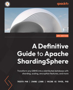
SQL Federation Engine is a crucial element not only in the implementation of data sharding but in the overall ShardingSphere ecosystem. The following diagram provides an overview of the SQL Federation Engine processes. This will give you a bird's-eye view of the whole process before we dive into the details:

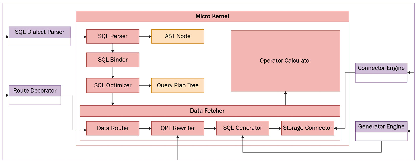
Figure 3.5 – The SQL Federation Engine processes

The SQL Federation Engine includes processes such as SQL Parser, Abstract Syntax Tree (AST), SQL Binder, SQL Optimizer, Data Fetcher, and Operator Calculator, which are used to process association queries and sub-queries across multiple database instances. The bottom layer uses calculations to optimize the Rule-Based Optimizer (RBO) and Cost-Based Optimizer (CBO) based on relational algebra, and query results through the optimal execution plan.

SQL Optimizer is responsible for optimizing the association query and sub-query across multiple database instances, as well as performing rule-based optimization and cost-based optimization to obtain the optimal execution plan.

Data Fetcher is responsible for obtaining data from the storage node according to the SQL that was generated by the optimal execution plan. Data Fetcher also routes, rewrites, and executes the generated SQL.

Leveraging the optimal execution plan and the data obtained from the storage node, the Operator Calculator is responsible for obtaining the query results and returning them to the user.

Why you need sharding

At this point, you have developed an understanding of the concept of data sharding and its key elements. Nevertheless, you may not know what the applications of data sharding are, nor the motivations that may prompt a DBA to implement data sharding. ShardingSphere's data sharding function provides transparent database shards and table shards. You can use the ShardingSphere data sharding function as if you were using a native database. At the same time, ShardingSphere provides a perfect distributed transaction solution, and users can manage distributed transactions in a unified way.

Moreover, combined with scaling, it can realize the elastic expansion of data sharding and ensure that the system can be continuously adjusted with the business, to meet the needs of rapid business growth. Nevertheless, sharding alone is not the solution to all the database issues of today, nor is it the only functionality provided by Apache ShardingSphere. The next section will introduce you to the SQL optimization feature.

Understanding SQL optimization

In a database management system, SQL optimization is crucial. The effect of SQL optimization is directly correlated to the execution efficiency of SQL statements. Therefore, current mainstream relational databases provide some type of powerful SQL optimizer. Based on traditional relational databases, ShardingSphere provides distributed database solutions that include data sharding, read/write splitting, distributed transactions, and other functions.

To meet the associated queries and subqueries across multiple database instances in distributed scenarios, ShardingSphere provides built-in SQL optimization functions through the federation execution engine. This helps achieve the optimal performance of query statements in distributed scenarios.

SQL optimization definition

SQL optimization refers to the equivalent transformation process for query statements and generating efficient physical execution plans using query optimization technology, which usually includes logical optimization and physical optimization:

• Logical optimization is RBO and refers to the equivalent transformation rules based on relational algebra to optimize query SQL, including column clipping, predicate pushdown, and other optimization contents.
• Physical optimization is CBO and refers to optimizing query SQL based on cost, including table connection mode, table connection order, sorting, and other optimization contents.

Now, let's learn more about RBO and CBO.

RBO

RBO refers to rule-based optimization. The theoretical basis of RBO is relational algebra. It realizes the logical optimization of SQL based on the equivalent transformation rules of relational algebra. It accepts a logical relational algebraic expression before returning the logical relational expression after rule transformation.

The main strategy of ShardingSphere logic optimization is to push down. For example, as shown in the following diagram, pushing the filter condition in an associated query join down to the internal execution of the join operation can effectively reduce the amount of data in the join operation:

Figure 3.6 – RBO explained

Additionally, considering that the underlying storage of ShardingSphere has computing power, Filter and Tablescan can be pushed down to the storage layer for execution at the same time, to further improve execution efficiency.

CBO

CBO refers to cost-based optimization. The SQL optimizer is responsible for estimating the cost of the query according to the cost model so that you can select the execution plan with the lowest cost per query. The following diagram shows an example of this:

Figure 3.7 – CBO explained

In traditional relational databases, cost estimation is usually based on CPU cost and I/O cost, while SQL optimization in ShardingSphere belongs to distributed query optimization, which makes reducing the number of transmissions and the amount of data as the main goal of query optimization. Therefore, in addition to CPU cost and I/O cost, the communication cost between different data nodes is also considered.

CBO optimization inputs a logical relational algebraic expression and returns the physical relational algebraic expression after optimization.

At the time of writing, ShardingSphere CBO optimization does not introduce statistical information. Instead, it uses the Calcite VolcanoPlanner optimizer to realize the transformation from a logical relational algebraic expression to a physical relational algebraic expression.

Note

Currently, the ShardingSphere SQL optimizer is still an experimental function and needs optimization in terms of performance and memory usage. Therefore, this function is turned off by default. Users can turn this function on by configuring sql-federation-enabled: true.

The value of SQL optimization

Through its SQL optimization function, ShardingSphere can support distributed query statements across multiple database instances and provide an efficient query performance guarantee.

At the same time, business R&D personnel no longer need to care about the purpose of SQL, as SQL is automatically optimized across multiple database instances. Also, they can focus on business function development and reduce the functional restrictions at the business level.

You have now gained an understanding of how ShardingSphere optimizes SQL through Simple Push Down and SQL Federation. These are important as SQL represents the way we interact with a database. In the next section, we will learn about one of the features where you will find this information useful: distributed transactions.

Overview and characteristics of distributed transactions

Transactions are important functions for database systems. A transaction is a logical unit that operates on a database and contains a collection of operations (generally referred to as SQL). When executing this transaction, it should hold ACID properties:

• Atomicity: All the operations in the transaction succeed or fail (be it read, write, update, or data deletion).
• Consistency: The status before and after the transaction's execution meets the same constraint. For example, in the classic transfer business, the account sum of the two accounts is equal before and after the transfer.
• Isolation: When transactions are executed concurrently, isolation acts as concurrency control. It ensures that the transaction's execution impacts the database in the same way as sequentially executed transactions would.
• Durability: By durability, we refer to the insurance that any changes that are made to the data by successfully executed transactions will be saved, even in cases of system failure (such as a power outage).

For a single-point database, it is convenient to support transactions on a physical node. For a distributed database system, a logical transaction may correspond to the operation of multiple physical nodes. Not only should each physical node provide transaction support, but there should also be a coordination mechanism to coordinate the transactions on multiple physical nodes and ensure the correctness of the whole logical transaction.

In the next few sections, you will understand how ShardingSphere supports both CAP and BASE theory through both rigid and flexible transactions. You will learn the difference between the two, as well as the differences between ShardingSphere's local, distributed, and flexible transactions.

Distributed transactions

Based on the CAP and BASE theories, distributed transactions are generally divided into rigid transactions and flexible transactions:

• Rigid transactions represent the strong consistency of the data.
• Flexible transactions represent the final consistency of the data.

The implementation method for distributed transactions has three roles:

• Application program (AP): This is an application that initiates logical transactions.
• Transaction manager (TM): A logical transaction will have multiple branch transactions to coordinate the execution, commit, and rollback of branch transactions.
• Resources manager (RM): This role executes branch transactions.

Considering distributed transactions' three roles, these are performed while following a two-phase submission:

1. Preparation phase:
   • TM informs RM to perform the relevant operations in advance.
   • RM checks the environment, locks the relevant resources, and executes them. If the execution is successful, it is in the prepared state and not in the completed state, and TM is notified of the execution result.
2. Commit/rollback phase:
   • If TM receives all the results that are returned by RM as successful, it will notify RM to submit the transaction.
   • Otherwise, TM will notify RM to roll back.

     Note

     Saga transaction and two-phase submission are very similar. The difference is that in the preparation phase, if the execution is successful, there is no prepared state.

If it is a read-committed (RC) isolation level, it is already visible to other transactions. When the rollback is executed, a reverse operation will be performed to roll the transactions back to their original states.

Note

Relevant logs will be recorded on both the TM and RM sides to deal with the problem of fault tolerance.

ShardingSphere's support for transactions

As discussed in the previous section, ShardingSphere supports rigid and flexible transactions. It encapsulates a variety of TM implementations through a pluggable architecture and provides you with the interface for begin/commit/rollbacks so that users do not need to care about additional configurations.

When one logical SQL hits multiple storage databases, it ensures the details of the transaction characteristics of multi-branch operations. This helps consistently convey the message across databases. The ShardingSphere transaction architecture is as follows:

Figure 3.8 – ShardingSphere transaction architecture

ShardingSphere's transaction manager is complete and greatly simplifies your configuration across multiple DBs to help you set up distributed transactions. The next few sections will introduce the different transaction types in detail.

Local transaction

A local transaction is based on the transaction of the underlying database. The distributed transaction can support the submission of cross-database transactions and the rollback that's caused by logical errors. Because there is no transaction maintaining the intermediate state, if there are network and hardware-related exceptions during the execution of a transaction, data may be inconsistent.

XA transaction

For XA transactions, two implementations of the open source transaction managers, atomic and Narayana, are integrated to ensure maximum data protection and avoid corruption. Based on the two-phase submission and the XA interface (which we first mentioned in Chapter 2, Architectural Overview of Apache ShardingSphere) of the underlying database, you must maintain the transaction log in the intermediate state, which can support distributed transactions.

At the same time, if problems are caused by unresponsive hardware (such as in case of a power outage or crash), the network, and exceptions, the proxy can roll back or commit the transactions in the intermediate state according to the transaction log.

Moreover, you can configure shared storage to store transaction logs (such as using MySQL to store transaction logs). By deploying the cluster mode of multiple proxies, you can increase the performance of proxies and support distributed transactions that include multiple proxies.

Flexible transaction

SEATA's Saga model transaction is integrated to provide a flexible transaction based on compensation. If an exception or error occurs in each branch transaction, the global transaction manager performs the opposite compensation operation and rolls back through the maintained transaction log to achieve the final consistency.

You have now reviewed the definitions and characteristics of all local, distributed, and flexible transactions – but what are the differences between them? Could you pinpoint some key parameters to differentiate them by? The next section will give you the knowledge to do just that.

Transaction modes comparison

The following table compares local, XA, and flexible transactions in terms of business transformation, consistency, isolation, and concurrent performance:

Table 3.1 – Transaction modes comparison

If you consider the comparison shown in the preceding table, you will probably be wondering which transaction type will fit which scenario. Depending on the type of scenario you are faced with, you can refer to the following rules of thumb:

• If the business can handle data inconsistencies caused by local transactions that have high-performance requirements, then local transaction mode is recommended.
• If strong data consistency and low concurrency are required, XA transaction mode is an ideal choice.
• If certain data consistency can be sacrificed, the transaction is large, and the concurrency is high, then flexible transaction mode is a good choice.

You now understand the three types of transactions, understand their defining characteristics, and have acquired rules of thumb to determine their suitability in certain scenarios. In the next section, we will introduce you to a scenario that DBAs are increasingly likely to encounter, thus increasing pressure on business support systems.

An introduction to elastic scaling

For a fast-growing business, support systems are generally under pressure, and all the layers of the hardware and software systems may become bottlenecks. In serious cases, there may be problems such as high system load, response delay, or even inability to provide services, thus affecting the user experience and causing the enterprise to incur losses.

From a system perspective, this is a high availability issue. The general solution is simple and direct. The system's pressure issues that are caused by insufficient resources (for example, insufficient storage capacity) can be solved by increasing resources, while excess resources can be solved by reducing resources. This process belongs to capacity expansion and contraction – that is, elastic scaling.

There are two types of expansion and contraction schemes in the industry – vertical scaling and horizontal scaling:

• Vertical scaling can be achieved by upgrading the single hardware. Affected by Moore's law, which states that the number of transistors on a microchip doubles approximately every 2 years, as well as by hardware costs, with you having to continuously upgrade single hardware, the marginal benefit of this scheme decreases. To solve this problem, the database industry has developed a horizontal scaling scheme.
• Horizontal scaling can be achieved by increasing or decreasing ordinary hardware resources. Although horizontal scaling interests hardware, the current state of applications in the computing layer has become relatively mature, and horizontal scaling can be well supported by the Share-Nothing architecture. This architecture is a typical architecture for distributed computing since, thanks to its design, each update is satisfied by a single node in the compute cluster.

Currently, elastic scaling is mainly used by the Apache ShardingSphere Proxy solution. Proxy products include a computing layer and storage layer, and both support elastic scaling. The storage layer is the underlying database that's supported by Apache ShardingSphere, such as MySQL and PostgreSQL. The storage layer is stateful, which brings some challenges to elastic scaling.

Glossary

Node: Instances of the computing layer or storage layer component processes can include physical machines, virtual machines, containers, and more.

Cluster: Multiple nodes grouped to provide specific services.

Data migration: Data migration moves data from one storage cluster to another.

Source end: The storage cluster where the original data resides.

Target end: The target storage cluster where the original data will be migrated.

Mastering elastic scaling

So far, you have learned about horizontal and vertical scaling. Elastic scaling, on the other hand, is the ability to automatically and flexibly add, reduce, or even remove compute infrastructure based on the changing requirement patterns dictated by traffic. On the data target side, elastic scaling can be divided into migration scaling and autoscaling. If the target is a new cluster, it is migration scaling. If the target end is a new node of the original cluster, it is auto-scaling. At the time of writing, Apache ShardingSphere supports migration scaling, and auto-scaling is under planning.

In migration scaling, we migrate all the data in the original storage cluster to the new storage cluster, including stock data and incremental data. Data migration to a new storage node takes some time and during the preparation period, the new storage node is unavailable.

How to ensure data correctness, enable the new storage node quickly, enable the new storage node smoothly, and make it so elastic scaling does not affect the operation of the existing system as much as possible are the challenges that are faced by storage layer elastic scaling.

Apache ShardingSphere provides corresponding solutions to these challenges. The implementation method will be described in the following section.

In addition, Apache ShardingSphere also provides good support in the following aspects:

• Operation convenience: Elastic scaling can be triggered by DistSQL, and the operation experience is the same as that of SQL. DistSQL is an extended SQL designed by Apache ShardingSphere, which provides a unified capability extension on the upper layer of a traditional database.
• Degree of freedom of the sharding algorithm: Different sharding algorithms have different characteristics. Some are conducive to data range queries, while others are conducive to data redistribution. Apache ShardingSphere supports rich types of sharding algorithms. In addition to modulus, hash, range, and time, it also supports user-defined sharding algorithms.

We will discuss these concepts in detail in Chapter 8, Apache ShardingSphere Advanced Usage – Database Plus and Plugin Platform. All sharding algorithms support elastic scaling.

The workflow to implement elastic scaling

Having introduced the concepts of vertical and horizontal scaling, let's review how to implement elastic scaling with ShardingSphere. Your general operation process will look like this:

1. Configure automatic switching configuration, data consistency verification, current limiting, and so on.
2. Trigger elastic scaling through DistSQL – for example, modify the sharding count through the ALTER SHARDING TABLE rule.
3. View your progress through DistSQL. Receive a failure alarm or success reminder.

Once elastic scaling has been triggered with ShardingSphere, the main workflow of the system will be as follows:

1. Stock data migration: The data originally located in the source storage cluster is stock data. Stock data can be extracted directly and then imported into the target storage cluster efficiently.
2. Incremental data migration: When data is migrated, the system is still providing services, and new data will enter the source storage cluster. This part of the new data is called incremental data and can be obtained through change data capture (CDC) technology, and then imported into the target storage cluster efficiently.
3. Detection of an incremental data migration progress: Since incremental data changes dynamically, we need to select the time point where there is no incremental data for subsequent steps to reduce the impact on the existing system.
4. Read-only mode: Set the source storage cluster to read-only mode.
5. Compare the data for consistency: Compare whether the data in the target end and the source end are consistent. The current implementation is at this stage and the new version will be optimized.
6. Target storage cluster: Switch configuration to the new target storage cluster by specifying the data source and rules.

The following diagram shows these steps:

Figure 3.9 – ShardingSphere elastic scaling workflow

The elastic scaling workflow will appear to be straightforward to you as ShardingSphere will handle the necessary steps. As shown in the preceding diagram, the required setup is fairly straightforward, and you only have to interact with the system for the Rule Configuration and, if desired, to query the Status.

Elastic scaling key points

Scheduling is the basis of elastic scaling. Data migration tasks are divided into multiple parts for parallel execution, clustered migration, automatic recovery after migration exceptions, online encryption and desensitization, and process scheduling at the same time, which are supported by the scheduling system.

Apache ShardingSphere uses the following methods to ensure the correctness of data:

• Data consistency verification: This compares whether the data at the source end and the data at the target end are consistent. If the data at both ends is inconsistent, the system will judge that elastic scaling failed and will not switch to a new storage cluster, to ensure that bad data will not go online. The data consistency verification algorithm supports SPI customization.
• The source storage cluster is set to read-only: The incremental data changes dynamically. To confirm that the data at both ends is completely consistent, a certain write stop time is required to ensure that the data does not change. The time taken to stop writing is generally determined by the amount of data, the arrangement of the verification process, and the verification algorithm.

Apache ShardingSphere smoothly enables new storage clusters by using an online switching configuration, including data sources and rules. The schema can be kept unchanged, and all proxy cluster (computing layer) nodes can be refreshed to the latest metadata so that the client can continue to be used normally without any operation.

Generally, the most time-consuming part of the process is data migration. The larger the amount of data, the greater the time consumption. Apache ShardingSphere uses the following incremental functions to enable new storage clusters faster:

• The data migration task is divided into multiple parts and executed in parallel.
• The modification operations of the same record are merged (for example, 10 update operations are merged into one update operation).
• We utilize a batch data import to improve speed by dividing the data into batches to not overload the system.
• We have a breakpoint resume transmission feature to ensure the continuity of data transfers in case of an unexpected interruption.
• Cluster migration. This function is under planning and hasn't been completed at the time of writing.

Apache ShardingSphere uses the following methods to minimize the impact on the operation of existing systems:

• Second-level read-only and SQL recovery: Regardless of the amount of data, most of it reaches second-level read-only. At the same time, SQL execution is suspended during read-only and is automatically recovered after writing stops, which does not affect the system's availability. At the time of writing, this is under development and hasn't been released yet.
• Rate limit: Limit the consumption of system resources via elastic scaling. At the time of writing, this is under development and hasn't been released yet.

These incremental functions are implemented based on the pluggable architecture of Apache ShardingSphere, which was first introduced in Figure 2.5 in Chapter 2, Architectural Overview of Apache ShardingSphere. The pluggable model is divided into three layers: the L1 kernel layer, the L2 function layer, and the L3 ecological layer. Elastic scaling is also integrated into the three-layer pluggable model, which is roughly layered as follows:

• Scheduling: Located in the L1 kernel layer, this includes task scheduling and task arrangement. It provides support for upper-layer functions such as elastic scaling, online encryption and desensitization, and MGR detection, and will support more functions in the future.
• Data ingestion: Located in the L1 kernel layer, this includes stock data extraction and incremental data acquisition. It supports upper-layer functions such as elastic scaling and online encryption and desensitization, with more features to be supported in the future. 
• The core process of the data pipeline: Located in the L1 kernel layer, this includes data pipeline metadata and reusable basic components in each step. It can be flexibly configured and assembled to support upper-layer functions such as elastic scalability and online encryption and desensitization. More features will be supported in the future.
• Elastic scaling, online encryption, and desensitization: Located in the L2 function layer, it reuses the L1 kernel layer and achieves lightweight functions through configuration and assembly. The SPI interface of some L1 kernel layers is realized through the dependency inversion principle.
• Implementation of database dialect: Located in the L3 ecological layer, it includes source end database permission checks, incremental data acquisition, data consistency verification, and SQL statement assembly.
• Data source abstraction and encapsulation: These are located in the L1 kernel layer and the L2 function layer. The basic classes and interfaces are located in the L1 kernel layer, while the implementation based on the dependency inversion principle is located in the L2 function layer.

  Note

  Elastic scaling is not supported in the following events:

  • If a database table does not have a primary key
  • If the primary key of a database table is a composite primary key
  • If there is no new database cluster at the target end

You are now an elastic scaling master in the making! You're only missing a playing field – that is, how and which real-world issues can you solve with elastic scaling? Read on to learn more.

How to leverage this technology to solve real-world issues

In the preceding sections, we talked about how increased pressure on systems may cause databases to become bottlenecks within an organization. As a solution, we have proposed elastic scaling, a technology that has gained widespread approval. What would be the typical application scenarios for this technology? Or, better yet, would you like to receive some real-world examples where this technology can be applied?

If that's the case, then please read on.

Typical application scenario 1

If an application system is using a traditional single database, with an amount of single-table data that has reached 100 million and is still growing rapidly, the single database continues to be under a high level of pressure, becoming a system bottleneck. Once the database becomes a bottleneck, expanding the application server becomes invalid, and the database needs to be expanded.

In this case, Apache ShardingSphere Proxy can provide help through the following general process:

1. Adjust the proxy configuration so that the existing single database becomes the storage layer of the proxy.
2. The application system will connect to the proxy and use the proxy as a database.
3. Prepare a new database cluster, and install and start the database instance.
4. Adjust the sharding count according to the hardware capability of the new database cluster to trigger the elastic scaling of Apache ShardingSphere.
5. Perform complete database cluster switching through Apache ShardingSphere's elastic scaling function.

Typical application scenario 2

If we expand the database according to scenario 1, but the number of users and visits has increased three times and continues to grow rapidly, the database load continues to be high, creating a system bottleneck, and we must continue to expand the database.

In this case, Apache ShardingSphere Proxy can help. The process is similar to scenario 1:

1. According to the historical data growth rate, plan how many database nodes are required in the next period (such as 1 year), prepare hardware resources, and install and start the database instance.
2. The following steps are the same as steps 4 and 5 of scenario 1.

Typical application scenario 3

If an application system contains some sensitive data saved in plaintext, to protect the user's sensitive data, even in the case of data leakage, it is necessary to encrypt the data.

In this case, Apache ShardingSphere Proxy can help encrypt and save the stock of sensitive data and subsequent new, sensitive data. It can be completed through the following general process:

1. Similar to scenario 1, first, configure and run the proxy.
2. Add the encrypted rule through DistSQL and configure the encryption option to trigger the Apache ShardingSphere encryption function.
3. Finish encrypting stock data and incremental data through Apache ShardingSphere's online encryption function.

With the last application scenario fully grasped, you now understand elastic scaling and Apache ShardingSphere's implementation of this technology. Now, you are ready to either apply your elastic scaling knowledge to your data environment. Alternatively, you can continue reading and learn more about ShardingSphere's features.

If you have chosen the second option, then please read on to learn more about r ead/write splitting.

Read/write splitting

With the growth of business volume, many applications will encounter the bottleneck of database throughput. It is difficult for a single database to carry a large number of concurrent queries and modifications. At the time of writing, a database cluster with primary-secondary configuration has become an effective scheme. Primary-secondary configuration means that the primary database is responsible for transactional operations such as data writing, modification, and deletion, while the secondary database is responsible for the database architecture of query operations.

The database with the primary-secondary configuration can limit the row lock that's brought by write operations to the primary database and support a large number of queries through the secondary database, greatly improving the performance of the application. Additionally, the multi-primary and multi-secondary database configuration can be adopted to ensure that the system is still available, even if the data node is down and if the database is physically damaged.

However, while the primary-secondary configuration brings the advantages of high reliability and high throughput, it also brings many problems.

The first is the inconsistency of the primary-secondary database data. Because the primary database and the secondary database are asynchronous, there must be a delay in database synchronization, which easily causes data inconsistency.

The second is the complexity brought by database clusters. Database operators, maintenance personnel, and application developers are facing increasingly complex systems. They must consider the configuration of the primary-secondary database to complete business tasks or maintain the database. The following diagram shows the complex topology between the application system and the database when the application system uses data sharding and read/write separation at the same time:

Figure 3.10 – Read/write splitting between databases

Here, we can see that the database cluster is very complex. To solve these complex problems, Apache ShardingSphere provides the read/write splitting function, allowing users to use the database cluster with primary-secondary configuration just as if they were using the native database.

Read/write splitting definition

Read/write splitting refers to routing the user's query operations and transactional write operations to different database nodes to improve the performance of the database system. Read/write splitting supports using a load balancing strategy, which can distribute requests evenly to different database nodes.

In the following sections, we will learn about the key points of the read/write splitting function, see how it works, and check out a few scenarios where this module has been applied.

Key points regarding the read/write splitting function

The read/write splitting function of Apache ShardingSphere includes many database-related concepts, including primary database, secondary database, primary-secondary synchronization, and load balancing strategy.

• Primary database refers to the database that's used for adding, updating, and deleting data. At the time of writing, only a single primary database is supported. 
• Secondary database refers to the database that's used for query data operation, which can support multiple secondary databases. 
• Primary-secondary synchronization refers to asynchronously synchronizing data from the primary database to the secondary database. Due to the asynchrony of primary-secondary database synchronization, the data of the secondary database and primary database will be inconsistent for a short time. 
• A load balancing strategy is used to divert query requests to different secondary databases.

How it works

The Apache ShardingSphere read/write splitting module parses the SQL input from the user through the SQL parsing engine and extracts the parsing context. The SQL routing engine identifies whether the current statement is a query statement according to the parsing context, to automatically route the SQL statement to the primary database or secondary database. The SQL execution engine will execute the SQL statement according to the routing results and is responsible for sending SQL to the corresponding data node for efficient execution. ShardingSphere's read/write splitting module has a variety of load balancing algorithms built into it, so that requests can be evenly distributed to each database node, effectively improving the performance and availability of the system.

The following diagram shows the different routing results of two different semantic SQLs. Here, we can see that read operations and write operations are routed to the secondary database and the primary database, respectively. For transactions containing both read and write operations, the ShardingSphere read/write splitting module will also route the corresponding SQL to the primary database to avoid data inconsistency:

Figure 3.11 – Semantic SQL routing results

Application scenarios

With the exponential growth of data volume, the linear growth brought by Moore's law to chip performance has made it increasingly difficult to meet users' needs in terms of performance, especially in the internet and financial industries.

To solve this problem, architecture adjustment has become the go-to solution. The read/write splitting architecture is favored by many companies because of its high availability and high performance.

To mitigate the cost increase caused by read/write splitting, Apache ShardingSphere can effectively reduce the complexity of read/write splitting, and let users use the database cluster with a primary-secondary configuration, similar to using a database.

Its built-in load balancing strategy can balance the load of each secondary database, to further improve system performance. In addition, the read/write splitting function of Apache ShardingSphere can be used in combination with its sharding function to further reduce the load and take the performance of the whole system to a new level.

The application scenarios for read/write splitting are truly numerous and understanding this feature will prove to be very useful to you.

Summary

In this chapter, you learned about the pluggable architecture of Apache ShardingSphere and started exploring the features that make up this architecture. By exploring features such as distributed databases, data sharding, SQL optimization, and elastic scaling, you now understand the component-based nature of Apache ShardingSphere.  

This project was built to provide you with any feature you may need, without imposing features on you that you may not need, thus giving you the power to build a ShardingSphere. You are now gaining the necessary knowledge to make informed decisions about which features to include in your version.

Since this chapter focused on the main features that will be necessary to build your distributed database and perform data sharding, in the next chapter, we will introduce the remaining major features that make up Apache ShardingSphere.