3
Compute and Networking
Several large and small organizations run workloads on AWS using AWS compute. Here, AWS Compute refers to a set of services on AWS that help you build and deploy your own solutions and services; this can include workloads as diverse as websites, data analytics engines, Machine Learning (ML), High-Performance Computing (HPC), and more. Being one of the first services to be released, Amazon Elastic Compute Cloud (EC2) is sometimes used synonymously with the term compute and offers a wide variety of instance types, processors, memory, and storage configurations for your workloads.
Apart from EC2, compute services that are suited to some specific types of workloads include Amazon Elastic Container Service (ECS), Elastic Kubernetes Service (EKS), Batch, Lambda, Wavelength, and Outposts. Networking on AWS refers to foundational networking services, including Amazon Virtual Private Cloud (VPC), AWS Transit Gateway, and AWS PrivateLink. These services, along with the various compute services, enable you to build solutions with the most secure and performant networked systems at a global scale. AWS compute and networking concepts are two broad topics and are important to understand many concepts that will be discussed in the following chapters.
Compute and networking also form two important pillars of HPC, along with data management, which was discussed in the last chapter. Every application of HPC is generally optimized for high levels of distributed compute, which depends on networking.
In this chapter, you will learn about the different services AWS offers for compute and networking, how these services are used for different types of computing workloads, and lastly, best practices for the HPC type of workloads on AWS, which goes beyond the AWS Well-Architected Framework.
Specifically, in this chapter, we will cover the following topics:
- Introducing the AWS compute ecosystem
- Networking on AWS
- Selecting the right compute for HPC workloads
- Best practices for HPC workloads
Introducing the AWS compute ecosystem
Compute lies at the foundation of every HPC application that you will read about in and outside of this book. In AWS and other clouds in general, compute refers to a group of services that offer the basic building blocks of performing a computation or some business logic. This can range from basic data computations to ML.
The basic units of measuring compute power on AWS (regardless of the service we are talking about) are as follows:
- Processing units – this can be measured as the number of Central Processing Units (CPUs), Virtual CPUs (vCPUs), or Graphics Processing Units (GPUs)
- Memory – this is the total requested or allocated memory for the application measured in units of bytes
Typical HPC applications access multiple instances and hence can take advantage of pooled compute and memory resources for larger workloads.
The foundational service that provides compute resources for customers to build their applications on AWS is called Amazon EC2. Amazon EC2 provides customers with a choice of about 500 instance types (at the time of writing this book and according to public documentation). Customers can then tailor the right combination of instance types for their business applications.
Amazon EC2 provides five types of instances:
- General purpose instances
- Compute optimized instances
- Accelerated computing instances
- Memory optimized instances
- Storage optimized instances
Each of the instance types listed here is actually a family of instances, as shown in Figure 3.1:
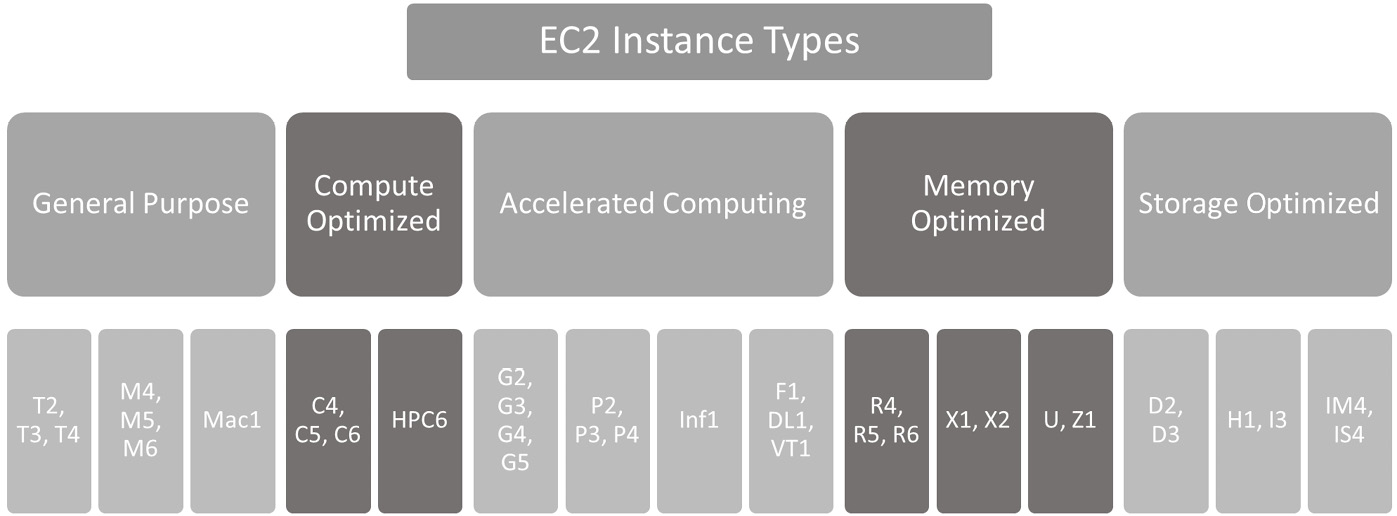
Figure 3.1 – Amazon EC2 instance types
In the following section, we will highlight some important facts about these instance types.
General purpose instances
General purpose instances can be used for a variety of workloads. They have the right balance of compute, memory, and storage for most typical applications that customers have on AWS. On AWS, there are several types of general purpose instances:
- T-type instances: T instances, for example, the T2 instance, are burstable instances that provide a basic level of compute for low compute- and memory-footprint workloads. The following figure shows what a typical workload that is suited for T-type instances might look like – most of the time is spent under the baseline CPU utilization level, with a need to burst above this baseline occasionally. With non-burstable instances, application owners need to over-provision for the burst CPU levels, and therefore pay more while utilizing very little. With burstable T instances, credits are accrued for utilization under the baseline (white areas below the baseline), and these credits can be used when the application is experiencing higher loads; see the gray filled-in areas in the following graph:

Figure 3.2 – CPU utilization versus time for burstable T-type instances on AWS
- M-type instances: M instances (like the M4, M5, and M6) can be used for a variety of workloads that need a balance of compute, memory, and networking, including (but not limited to) web and application servers, and small to medium-sized database workloads. Special versions of M5 and M6 instances are offered that are suitable for certain workloads. For example, the M5zn instance types can be used for applications that demand extremely high single-threaded performance, such as HPC, simulations, and gaming.
- A-type instances: A1 instances are used to run Advanced RISC Machine or ARM-based applications, such as microservices and web servers powered by the AWS Graviton ARM processors.
- Mac-type instances: Mac1 instances are powered by Apple’s Mac Mini computers and provide very high network and storage bandwidth. They are typically used for building and testing Apple applications for the iPhone, Mac, and so on.
In the following section, we will discuss compute optimized instances on AWS.
Compute optimized instances
Many HPC applications that will be described in this book take advantage of the high-performance, compute optimized instance types on AWS.
There are several types of compute optimized instances:
- C5 instances: C5 and C5n instances provide low-cost, high-performance compute for typical HPC, gaming, batch processing, and modeling. C5 instances use Intel Xeon processors (first and second generation) and provide upward of 3.4 GHz clock speeds on a single core. C5a instances also provide AMD processors for high performance at an even lower cost. C5n instances are well suited to HPC applications since they support Elastic Fabric Adapter (EFA) and can deliver up to 100 gigabits per second of networking throughput. For more information about EFA, please visit https://aws.amazon.com/hpc/efa/.
- C6 instances: C6g instances are ARM-based instances based on the AWS Graviton processor. They are ideal for running HPC workloads, ad serving, and game servers. C6g instances are available with local Non-Volatile Memory express or NVMe-based high performance, low latency SSD storage with 100 gigabits per second networking, and support for EFA. On the other hand, the C6i class of instances is Intel Xeon-based and can provide up to 128 vCPUs per instance for typical HPC workloads.
- HPC instances: The HPC6a instance type is powered by third-generation AMD processors for lower cost-to-performance ratios for typical HPC workloads. These instance types also provide 96 CPU cores and 384 GB of RAM for memory-intensive applications. HPC6a instances also support EFA-based networking for up to 100 gigabits per second of throughput.
In the following section, we will discuss accelerated compute instances on AWS.
Accelerated compute instances
Accelerated computing instances use co-processors such as GPUs to accelerate performance for workloads such as floating point number calculations useful for ML, deep learning, and graphics processing.
Accelerated compute instances use hardware-based compute accelerators such as the following:
- GPUs
- Field Programmable Gate Arrays (FPGAs)
- AWS Inferentia
GPUs
GPUs were originally used for 3D graphics but are now being used as general-purpose co-processors for various applications such as HPC and deep learning. HPC applications are computation and bandwidth-heavy. Several types of NVIDIA GPUs are available on AWS, and detailed information can be found at the following link, https://aws.amazon.com/nvidia/.
Let’s dive into the basics of how GPUs help with compute-heavy calculations. Imagine adding a list of numbers to another list of the same size. Visually, this looks like the following diagram:

Figure 2.3 – Adding two arrays
The naïve way of adding these to arrays is to loop through all elements of each array and add each corresponding number from the top and bottom arrays. This may be fine for small arrays, but what about arrays that are millions of elements long? To do this on a GPU, we first allocate memory for these two very long arrays and then use threads to parallelize these computations. Adding these arrays using a single thread on a single GPU is the same as our earlier naïve approach. Using multiple threads (say 256) can help parallelize this operation by allocating a part of the work to each thread. For example, the first few elements (the total size divided by 256 in this case) will be done by the first thread, and so on. This speeds up the operation by letting each thread focus on a smaller portion of the work and do each of these split-up addition operations in parallel; see the shaded region in the following diagram:

Figure 3.4 – Multiple threads handling a portion of the computation
GPUs today are architected in a way that allows even higher levels of parallelism – multiple processing threads make up a block, and there are usually multiple blocks in a GPU. Each block can run concurrently in a Streaming Multiprocessor (SM) and process the same set of computations or kernels. Visually, this looks like the following:

Figure 3.5 – Multiple blocks in a GPU
To give you an idea of what you can access on AWS, consider the P4d.24xlarge instance. This instance has eight GPUs, as seen in the following figure, each of which is an NVIDIA A100 housing 108 SMs, with each SM capable of running 2,048 threads in parallel:

Figure 3.6 – A single instance with multiple GPUs
On AWS, P4d instances can be used to provision a supercomputer or an EC2 Ultracluster with more than 4,000 A100 GPUs, Petabit-scale networking, and scalable, shared high throughput storage on Amazon FSx for Lustre (https://aws.amazon.com/fsx/lustre/). Application and package developers use the NVIDIA CUDA library to build massively parallel applications for HPC and deep learning. For example, PyTorch, a popular ML library, uses NVIDIA’s CUDA GPU programming library for training large-scale models. Another example is Ansys Fluent, a popular Computational Fluid Dynamics (CFD) simulation software that uses GPU cores to accelerate fluid flow computations.
On AWS, there are several families of GPU instances:
- G family of instances: G2, G3, G4, and G5 type instances on AWS provide cost-effective access to GPU resources. Each G-type instance mentioned here comes with a different NVIDIA GPU – for example, the latest G5 instances come with NVIDIA A10G GPUs, G5g instances with NVIDIA T4G GPUs, and G4Dn with the NVIDIA Tesla GPUs. AMD-based GPUs are also available – for example, the G4ad instances use the AMD Radeon Pro V520 GPUs.
- P family of instances: These instances provide extremely high-performance GPUs for single-instance and distributed applications. The P2 instances provide access to the NVIDIA K80 GPUs, P3 instances have the NVIDIA Tesla V100 GPUs, and the P4d instances have the A10 GPUs.
- VT1 instances: These provide access to the Xilinx Alveo U30 media accelerator cards that are primarily used for video transcoding applications. More information about VT1 instances can be found here: https://aws.amazon.com/ec2/instance-types/vt1/.
- AWS Inferentia: These instances are specifically designed to provide cost-effective and low latency ML inference capability and are a custom-made chip created by AWS. A typical workflow that customers could follow using these Inf1 instances is to use an ML framework like TensorFlow to train a model on another EC2 instance or SageMaker training instances, then use Amazon SageMaker’s compilation feature Neo to compile the model for use with the Inf1 instances. You can also make use of the AWS Neuron SDK to profile and deploy deep learning models onto Inf1 instances.
FPGA instances
Amazon EC2 F1 instances allow you to develop and deploy hardware-accelerated applications easily on the cloud. Example applications include (but are not limited to) big data analytics, genomics, and simulation-related applications. Developers can use high-level C/C++ code to program their applications, register the FPGA as an Amazon FPGA Image (AFI), and deploy the application to an F1 instance. For more information on F1 instances, please refer to the links in the Reference section at the end of this chapter.
In the following section, we will discuss memory optimized compute instances on AWS.
Memory optimized instances
Memory optimized instances on AWS are suited to run applications that require storage of extremely large data in memory. Typical applications that fall into this category are in-memory databases, HPC applications, simulation, and Electronic Design Automation (EDA) applications. On AWS, there are several types of memory optimized instances:
- R5 instances: The R5 family of instances (such as the R5, R5a, R5b, and R5n instance types) is a great choice for relational databases such as MySQL, MongoDB, and Cassandra, for in-memory databases such as Redis and Memcached, and business intelligence applications, such as SAP HANA and HPC applications. The R5 metal instance type also provides direct access to processors and memory on the physical server that the instance is based on.
- R6 instances: R6 instances such as R6g and R6gd are based on ARM-based AWS Gravitron2 processors and can provide better price-to-performance ratios compared to R5 instances. Application developers can use these instance types to develop or support ARM-based applications that need a high memory footprint.
- U instances: These instances are extremely high memory instances – they can offer anywhere from 6 to 24 TB of memory per instance. They are typically used to run large in-memory applications such as databases and SAP HANA and are powered by Intel Xeon Platinum 8176M processors.
- X instances: X-type instances (such as X1, X1e, and X1gd instance types) are designed for large-scale in-memory applications in the cloud. Each X1 instance is powered by four Intel Xeon E8880 processors with up to 128 vCPUs, and up to 1,952 GB of memory. X1 instances are picked by developers for their low price-to-performance ratio given the amount of memory provided, compared to other families of instances. X1e instances provide even higher memory (up to 3,904 GB) and support production-grade SAP workloads. Both X1 and X1e instance types provide up to 25 gigabits per second of network bandwidth when used with an Elastic Network Adapter (ENA). Finally, X1gd and X2gd are AWS Graviton2-based ARM instances that provide better price performance compared to x86-based X1 instances.
- Z instance types: The Z1d instance type provides both high performance and high memory for typical data analytics, financial services, and HPC applications. Z1d instances are well suited for applications that need very high single-threaded performance, with an added dependence on high memory. Z1d instances come in seven different sizes, and up to 48 vCPUs and 384 GB of RAM, so customers can choose the right instance size for their application.
Storage optimized instances
Storage optimized instances are well suited for applications that need frequent, sequential reads and writes from local storage by providing very high I/O Operations Per Second (IOPS). There are several storage optimized instances on AWS:
- D-type instances: Instances such as D2, D3, and D3en provide high-performance local storage and can be used for MapReduce-style operations (with Hadoop or Spark), log processing, and other big data workloads that do not require all the data to be held in memory but require very fast, on-demand access to this data.
- H-type instances: The H1 instance is typically used for MapReduce applications and distributed file storage, and other data-intensive applications.
- I-type instances: I type instances such as I3 and I3en are well suited for relational and non-relational databases, in-memory caches, and other big data applications. The I3 instances are NVMe Solid State Drive (SSD) -based instances that can provide up to 25 GB of network bandwidth and 14 gigabits per second of dedicated bandwidth to attached Elastic Block Store (EBS) volumes. The Im4gn and Is4gen type instances can be used for relational and NoSQL databases, streaming applications, and distributed file applications.
Amazon Machine Images (AMIs)
Now that we have discussed different instance types that you can choose for your applications on AWS, we can move on to the topic of Amazon Machine Images (AMIs). AMIs contain all the information needed to launch an instance. This includes the following:
- The description of the operating system to use, the architecture (32 or 64-bit), any applications to be included along with an application server, and EBS snapshots to be attached before launch
- Block-device mapping that defines which volumes to attach to the instance on launch
- Launch permissions that control which AWS accounts can use this AMI
You can create your own AMI, or buy, share, or sell your AMIs on the AWS Marketplace. AWS maintains Amazon Linux-based AMIs that are stable and secure, updated and maintained on a regular basis, and includes several AWS tools and packages. Furthermore, these AMIs are provided free of charge to AWS customers.
Containers on AWS
In the previous section, we spoke about AMIs on AWS that can help isolate and replicate applications across several instances and instance types. Containers can be used to further isolate and launch one or more applications onto instances. The most popular flavor of containers is called Docker. Docker is an open platform for developing, shipping, and running applications. Docker provides the ability to package and run an application in a loosely isolated environment called a container. Docker containers are definitions of runnable images, and these images can be run locally on your computer, on virtual machines, or in the cloud. Docker containers can be run on any host operating system, and as such are extremely portable, as long as Docker is running on the host system.
A Docker container contains everything that is needed to run the applications that are defined inside it – this includes configuration information, directory structure, software dependencies, binaries, and packages. This may sound complicated, but it is actually very easy to define a Docker image; this is done in a Dockerfile that may look similar to this:
FROM python:3.7-alpine
COPY . /app
WORKDIR /app
RUN pip install -r requirements.txt
CMD ["gunicorn", "-w 4", "main:app"]
The preceding file named Dockerfile defines the Docker image to run a sample Python application using the popular Gunicorn package (see the last line in the file). Before we can run the application, we tell Docker to use the Python-3.7 base image (FROM python:3.7-alpine), copy all the required files from the host system to a folder called app, and install requirements or dependencies for that application to run successfully (RUN pip install -r requirements.txt). Now you can test out this application locally before deploying it at scale on the cloud.
On AWS, you can run containers on EC2 instances of your choice or make use of the many container services available:
- When you need to run containers with server-level control, you can directly run the images that you define on EC2. Furthermore, running these containers on EC2 Spot instances can save you up to 90% of the cost over on-demand instances. For more information on Spot instances please refer to https://aws.amazon.com/ec2/spot/.
- At the opposite end of the spectrum, you can use a service like AWS Fargate to run containers without managing servers. Fargate removes all the operational overhead of maintaining server-level software so you can focus on just the application at hand. With Fargate, you only pay for what you use – for example, if you create an application that downloads data files from Amazon S3, processes these files, and writes output files back to S3, and this process takes 30 minutes to finish, you only pay for the time and resources (vCPUs) used to complete the task.
- When you have multiple, complex, container-based applications, managing and orchestrating these applications is an important task. On AWS, container management and orchestration can be achieved using services like Amazon Elastic Container Registry (ECR), Amazon Elastic Container Service (ECS), and Amazon Elastic Kubernetes Service (EKS). A detailed discussion about these services is outside the scope of this book but if you are interested, you can refer to the links mentioned in the References section to learn more.
Serverless compute on AWS
In the previous section, you read about AWS Fargate, which lets you run applications and code based on Docker containers, without the need to manage infrastructure. This is an example of a serverless service on AWS. AWS offers serverless services that have the following features in common:
- No infrastructure to manage
- Automatic scaling
- Built-in high availability
- Pay-per-use billing
Serverless compute technologies on AWS are AWS Lambda and Fargate. AWS Lambda is a serverless computing service that lets you run any code that can be triggered by over 200 services and SaaS applications. Code can be written in popular languages such as Python, Node.js, Go, and Java or can be packaged as Docker containers, as described earlier. With AWS Lambda, you only pay for the number of milliseconds that your code runs, beyond a very generous free tier of over a million free requests. AWS Lambda supports the creation of a wide variety of applications including file processing, streaming, web applications, IoT backend applications, and mobile app backends.
For more information on serverless computing on AWS, please refer to the links included in the References section.
In the next section, we will cover basic concepts around networking on AWS.
Networking on AWS
Networking on AWS is a vast topic that is out of the scope of this book. However, in order to easily explain some of the sections and chapters that follow, we will attempt to provide a brief overview here. First, AWS has a concept called regions, which are physical areas around the world where AWS places clusters of data centers. Each region contains multiple logically separated, groups of data centers called availability zones. Each availability zone has independent power, cooling, and physical security. Availability zones are connected via redundant and ultra-low latency AWS Networks. At the time of writing this chapter, AWS has 26 regions and 84 availability zones.
The next foundational concept we will discuss here is a Virtual Private Cloud (VPC). A VPC is a logical partition that lets you launch and group AWS resources. In the following diagram, we can see that a region has multiple availability zones that can span multiple VPCs:

Figure 3.7 – Relationship between regions, VPCs, and availability zones
A subnet is a range of IP addresses associated with the VPC you have defined. A route table is a set of rules that determine how traffic will flow within the VPC. Every subnet you create in a VPC is automatically associated with the main route table of the VPC. A VPC endpoint lets you connect resources from one VPC to another and to other services.
Next, we will discuss Classless Inter-Domain Routing (CIDR) blocks and routing.
CIDR blocks and routing
CIDR is a set of standards that is useful for assigning IP addresses to a device or group of devices. A CIDR block looks like the following:
10.0.0.0/16
This defines the starting IP, and the number of IP addresses in the block. Here, the 16 means that there are 2^(32-16) or 65,536 unique addresses. When you create a CIDR block, you have to make sure that all IP addresses are contiguous, the block size is a power of 2, and IPs range from 0.0.0.0 to 256.256.256.256.
For example, the CIDR block 10.117.50.0/22 has a total of 2^(32-22), or 1,024 addresses. Now, if we would like to partition this network into four more networks with 256 addresses each, we could use the following CIDR blocks:
|
10.117.50.0.22 |
10.117.50.0/24 |
256 addresses |
|
10.117.51.0/24 |
256 addresses | |
|
10.117.52.0/24 |
256 addresses | |
|
10.117.53.0/24 |
256 addresses |
Figure 3.8 – Example of using CIDR blocks to create four partitions on the network
Great, now that we know how CIDR blocks work, let us apply the same to VPCs and subnets.
Networking for HPC workloads
Referring back to Figure 3.8, we have made a few modifications to show CIDR blocks that define two subnets within VPC1 in the following diagram:

Figure 3.9 – CIDR blocks used to define two subnets within VPC1
As we can see in Figure 3.9, VPC 1 has a CIDR block of 10.0.0.0/16 (amounting to 65,536 addresses), and the two subnets (/24) have allocated 256 addresses each. As you have already noticed, there are several unallocated addresses in this VPC, which can be used in the future for more subnets. Routing decisions are defined using a route table, as shown in the figure. Here, each subnet is considered to be private, as traffic originating from within the VPC cannot leave the VPC. This also means that resources within this VPC cannot, by default, access the internet. One way to allow resources from within a subnet to access the internet is to add an internet gateway. For allowing only outbound internet connection from a private subnet, you can use an NAT gateway. This is often a requirement for security-sensitive workloads. This modification results in the following change to our network diagram:

Figure 3.10 – Adding an internet gateway to Subnet 1
The main route table is associated with all subnets in the VPC, but we can also define custom route tables for each subnet. This defines whether the subnet is private, public, or VPN only. Now, if we need resources in Subnet 2 to only access VPN resources in a corporate network via a Virtual Private Gateway (VGW) in Figure 3.11, we can create two route tables and associate them with Subnet 1 and Subnet 2, as shown in the following diagram:

Figure 3.11 – Adding a VGW to connect to on-premises resources
A feature called VPC peering can be used in order to privately access resources in another VPC on AWS. With VPC peering, you can use a private networking connection between two VPCs to enable communication between them. For more information, you can visit https://docs.aws.amazon.com/vpc/latest/peering/what-is-vpc-peering.html. As shown in the following diagram, VPC peering allows resources in VPC 1 and VPC 2 to communicate with each other as though they are in the same network:

Figure 3.12 – Adding VPC peering and VPC endpoints
VPC peering can be done within VPCs in the same region or VPCs in different regions. A VPC endpoint allows resources from within a VPC (here, VPC 2) to access AWS services privately. Here, an EC2 instance can make private API calls to services such as Amazon S3, Kinesis, or SageMaker. These are called interface-type endpoints. Gateway-type VPC endpoints are also available for Amazon S3 and DynamoDB, where you can further customize access control using policies (for example, bucket policies for Amazon S3).
Large enterprise customers with workloads that run on-premises, as well as on the cloud, may have a setup similar to Figure 3.13:

Figure 3.13 – Enterprise network architecture example
Each corporate location may be connected to AWS by using Direct Connect (a service for creating dedicated network connections to AWS with a VPN backup. Private subnets may host single or clusters of EC2 instances for large, permanent workloads. The cluster of EC2 instances is placed in a multi-AZ autoscaling group so that the workload can recover from the unlikely event of an AZ failure, and a minimum number of EC2 instances is maintained.
For ephemeral workloads, managed services such as EKS, Glue, or SageMaker can be used. In the preceding diagram, a private EKS cluster is placed in VPC 2. Since internet access is disabled by default, all container images must be local to the VPC or copied onto an ECR repository; that is, you cannot use an image from Docker Hub. To publish logs and save checkpoints, VPC endpoints are required in VPC 2 to connect to the Amazon S3 and CloudWatch services. Data stores and databases are not discussed in this diagram but are important considerations in hybrid architectures. This is because some data cannot leave the corporate network but may be anonymized and replicated on AWS temporarily.
Typically, this temporary data on AWS is used for analytics purposes before getting deleted. Lastly, hybrid architectures may also involve AWS Outposts, which is a fully managed service that extends AWS services, such as EC2, ECS, EKS, S3, EMR, Relational Database Service (RDS) and so on, to on-premises.
Selecting the right compute for HPC workloads
Now that you have learned about the foundations of compute and network on AWS, we are ready to explore some typical architectural patterns for compute on AWS.
Selecting the right compute for HPC and ML applications involves considering the rest of the architecture you are designing, and therefore involves all aspects of the Well-Architected Framework:
- Operational excellence
- Security
- Reliability
- Performance efficiency
- Cost optimization
We cover best practices across these pillars at the end of this section, but first, we will start with the most basic pattern of computing on AWS and add complexity as we progress.
Pattern 1 – a standalone instance
Many HPC applications that are built for simulations, financial services, CFD, or genomics can run on a single EC2 instance as long as the right instance type is selected. We discussed many of these instance-type options in the Introducing AWS compute ecosystem section. As shown in the following diagram, a CloudFormation Template can be used to launch an EC2 Instance in a VPC, and Secure Shell (SSH) access can be provided to the user for installing and using software on this instance:

Figure 3.14 – CloudFormation Template used to launch an EC2 Instance inside a VPC
Next, we will describe a pattern that uses AWS ParallelCluster.
Pattern 2 – using AWS ParallelCluster
AWS ParallelCluster can be used to provision a cluster with head and worker nodes for massive-scale parallel processing or HPC. ParallelCluster, once launched, will be similar to on-premises HPC clusters with the added benefits of security and scalability in the cloud. These clusters can be permanent or provisioned and de-provisioned on an as-needed basis. On AWS, a user can use the AWS ParallelCluster Command-Line Interface (CLI) to create a cluster of EC2 instances on the fly. AWS CloudFormation is used to launch the infrastructure, including required networking, storage, and AMI configurations. As the user (or multiple users) submit jobs through the job scheduler, more instances are provisioned and de-provisioned in the autoscaling group, as shown in the following diagram:
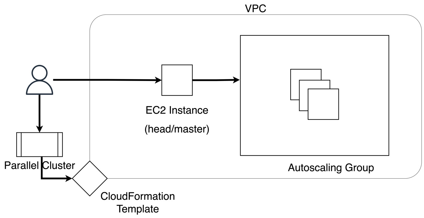
Figure 3.15 – Using AWS ParallelCluster for distributed workloads on AWS
Once the user is done with using the cluster for their HPC workloads, they can use the CLI or CloudFormation APIs to delete all resources created. As a modification to what is suggested in the following architecture, you can replace the head/master EC2 node with an Amazon SQS queue to get a queue-based architecture for typical HPC workloads.
Next, we will discuss how you can use AWS Batch.
Pattern 3 – using AWS Batch
AWS Batch helps run HPC and big data-based applications that are based on unconnected input configurations or files without the need to manage infrastructure. To submit a job to AWS batch, you package your application as a container and use the CLI or supported APIs to define and submit a job. With AWS Batch, you can get started quickly by using default job configurations, a built-in job queue, and integration with workflow services such as AWS Step Functions and Luigi.
As you can see in the following screenshot, the user first defines a Docker image (much like the image we discussed in the section on containers) and then registers this image with Amazon ECR. Then, the user can create a job definition in AWS Batch and submit one or more jobs to the job queue. Input data can be pulled from Amazon S3, and output data can be written to a different location on Amazon S3:

Figure 3.16 – Using AWS Batch along with AWS EC2 instances for batch workloads
Next, we will discuss patterns that help with hybrid architectures on AWS.
Pattern 4 – hybrid architecture
Customers who have already invested in large on-premises clusters, and who also want to make use of the on-demand, highly scalable, and secure AWS environment for their jobs, generally opt for a hybrid approach. In this approach, organizations decide to do one of the following:
- Run a particular job type on AWS and keep the rest on-premises
- Use AWS for overflow/excess capacity
- Use on-premises as primary data storage for security reasons, or place only the scheduler or job monitors on-premises with all of the compute being done on AWS
- Run small, test, or development jobs on-premises, but larger production jobs using high-performance or high-memory instances on AWS
On-premises data can be transferred to Amazon S3 using a software agent called DataSync (see https://docs.aws.amazon.com/datasync/latest/userguide/working-with-agents.html). Clusters that use Lustre’s shared high-performance file system on-premises can make use of Amazon FSx for Lustre on AWS (for more information, see https://aws.amazon.com/fsx/lustre/). The following diagram is a reference architecture for hybrid workloads:

Figure 3.17 – Using FSx, S3, and AWS DataSync for hybrid architectures
Next, we will discuss patterns for container-based distributed processing
Pattern 5 – Container-based distributed processing
The following diagram is a reference architecture for container-based distributed processing workflows that are suited for HPC and other related applications:

Figure 3.18 – EKS-based architecture for distributed computing
Admins can use command-line tools such as eksctl or CloudFormation to provision resources. Pods that are one or more containers can be run on managed EC2 nodes of your choice or via the AWS Fargate service. EMR on EKS can also be used to run open source, big data applications (for example, based on Spark) directly on EKS-managed nodes. In all of the preceding cases, containers that are provided by AWS can be used as a baseline, or completely custom containers that you build and push to ECR may be used. Applications running in EKS pods can access data from Amazon S3, Redshift, DynamoDB, or a host of other services and applications. To learn more about EKS, Fargate, or EMR on EKS, please take a look at the links provided in the References section.
Pattern 6 – serverless architecture
The following diagram is an example of serverless architecture that can be used for real-time, serverless processing, analytics, and business intelligence:

Figure 3.19 – Architecture for real-time, serverless processing and business analytics
First, Kinesis Data Streams captures data from one or more data producers. Next, Kinesis Data Analytics can be used to build real-time applications for transforming this incoming data using SQL, Java, Python, or Scala. Data can also be interactively processed using managed Apache Zeppelin notebooks (https://zeppelin.apache.org/). In this case, a Lambda Function is being used to continuously post-process the output of the Kinesis Analytics application before dropping a filtered set of results into the serverless, NoSQL database DynamoDB.
Simultaneously, the Kinesis Firehose component is being used to save incoming data into S3, which is then processed by several other serverless components such as AWS Glu and AWS Lambda, and orchestrated using AWS Step Functions. With AWS Glue, you can run serverless Extract-Transform-Load (ETL) applications that are written in familiar languages such as SQL or Spark. You can then save the output of Glue transform jobs to data stores such as Amazon S3 or Amazon Redshift. ML applications that run on Amazon SageMaker can also make use of the output data from real-time streaming analytics.
Once the data is transformed, it is ready to be queried interactively using Amazon Athena. Amazon Athena makes it possible for you to query data that resides in Amazon S3 using standard SQL commands. Athena is also directly integrated with the Glue Data Catalog, which makes it much easier to work with these two services without the additional burden of writing ETL jobs or scripts to enable this connection. Athena is built on the open source library Presto (https://prestodb.io/) and can be used to query a variety of standard formats such as CSV, JSON, Parquet, and Avro. With Athena Federated data sources, you can use a visualization tool such as Amazon QuickSight to run complex SQL queries.
Rather than using a dataset to visualize outputs, QuickSight, when configured correctly, can directly send these SQL queries to Athena. The results of the query can then be directly visualized interactively using multiple chart types and organized into a dashboard. These dashboards can then be shared with business analysts for further research.
In this section, we have covered various patterns around the topic of compute on AWS. Although this is not an exhaustive list of patterns, this should give you a basic idea of the components or services used and how these components are connected to each other to achieve different requirements. Next, we will describe some best practices related to HPC on AWS.
Best practices for HPC workloads
The AWS Well-Architected Framework helps with the architecting of secure, cost-effective, resilient, and high-performing applications and workloads on the cloud. It is the go-to reference when building any application. Details about the AWS Well-Architected Framework can be obtained at https://aws.amazon.com/architecture/well-architected/. However, applications in certain domains and verticals require further scrutiny and have details that need to be handled differently from the generic guidance that the AWS Well-Architected Framework provides. Thus, we have many other documents called lenses that provide best practice guidance; some of these lenses that are relevant to our current discussion are listed as follows:
- Data Analytics Lens – well-architected lens for data analytics workloads (https://docs.aws.amazon.com/wellarchitected/latest/analytics-lens/analytics-lens.html?did=wp_card&trk=wp_card)
- Serverless Lens – focusing on architecting serverless applications on AWS (https://docs.aws.amazon.com/wellarchitected/latest/serverless-applications-lens/welcome.html)
- ML Lens – for ML workloads on AWS (https://docs.aws.amazon.com/wellarchitected/latest/machine-learning-lens/welcome.html?did=wp_card&trk=wp_card)
- HPC Lens – focusing on HPC workloads on AWS (https://docs.aws.amazon.com/wellarchitected/latest/high-performance-computing-lens/welcome.html?did=wp_card&trk=wp_card)
While it is out of the scope of this book to go over best practices from the generic AWS Well-Architected Framework, as well as these individual lenses, we will list some common, important design considerations that are relevant to our current topic of HPC and ML:
- Both HPC and ML applications evolve over time. Organizations that freeze an architecture for several years in advance tend to be the ones that resist change and are later impacted by even larger costs to accommodate new requirements. In general, it is best practice to avoid static architectures, as the original requirements may evolve quickly. When there is a need to run more training jobs, or more HPC simulations, the architecture must allow scaling out and increase overall performance, but also return back to a steady, low-cost state when the demand is lower.
On AWS, compute clusters can be right-sized at any given point in time, and the use of managed services can help with provisioning resources on the fly. For example, Amazon SageMaker allows users to provision various instance types for training without the undifferentiated heavy lifting of maintaining clusters or infrastructure. Customers only need to choose the framework of interest, point to training data in Amazon S3, and use the APIs to start, monitor, and stop training jobs. Customers only pay for what they use and don’t pay for any idle time.
- Architecting to encourage and enable collaboration can make a significant difference to the productivity of the team running HPC and ML workloads on AWS. With teams that are becoming remote and global, the importance of effective collaboration cannot be understated. To improve collaboration, it is important to do the following:
- Track experiments using an experiment tracking tool.
- Enable sharing of resources such as configuration files, CloudFormation templates, pipeline definitions, code, notebooks, and data.
- Enable automation and use tools for continuous integration, continuous delivery, continuous monitoring, continuous training, and continuous improvement.
- Make sure that work is reproducible – this means that the inputs, environmental configuration, and packages can be easily reused and the outputs of a batch process can be verified. This helps to track changes, with audits, and to maintain high standards.
- Use ephemeral resources from managed services when possible. Again, this is applicable to both HPC and ML. When considering hybrid architectures or when migrating an on-premises workload to AWS, it is no longer necessary to completely replicate the workload on AWS. For example, running Spark-based workloads can be done on AWS Glue without the need to provision an entire EMR cluster. Similarly, you can run ML training or inference without handling the underlying clusters using Amazon SageMaker APIs.
- Consider both performance and cost when right-sizing your resources. For workloads that are not time-sensitive, using Spot instance on AWS is the simplest cost optimization strategy to follow. For HPC applications, running workloads on EC2 spot instances or using spot fleets for containerized workloads on EKS or Fargate can provide a discount of up to 90% over on-demand instances of the same type.
On SageMaker, using Spot instances is very simple – you just need to pass an argument to supported training APIs. On the other hand, for high-performance workloads, it is important to prioritize on-demand instances over spot instances so that the results of simulations or ML training jobs can be returned and analyzed in a timely manner. When choosing services or applications to use for your HPC or ML workloads, prefer pay-as-you-go pricing over licensing and upfront costs.
- Consider cost optimization and performance for the entire pipeline. It is typical for both HPC and ML applications to be designed over a pipeline – for example, data transfer, pre-processing, training or simulation, post-processing, and visualization. It is possible that some steps require less compute than others. Also, making a decision upfront about data formats or locations may force downstream steps to be more expensive in terms of time, processing resources, or cost.
- Focus on making small and frequent changes, building modular components, and testing in an automated fashion. Reducing the level of manual intervention and architecting the workload so that it does not require any downtown for maintenance is a best practice.
- For both HPC and ML, use software packages and tools that provide good documentation and support. This choice needs to be made carefully upfront, since several architectural, design, and team decisions may need to change based on this. For example, when choosing an ML framework such as PyTorch, it is important to be familiar with services on AWS that support this framework and hire a team that is well-versed in this particular framework to ensure success.
Similarly in HPC, the choice of software that does molecular dynamics simulations will decide the scale of simulations that can be done, which services are compatible with the package on AWS, and which team members are trained and ready to make use of this software set up on AWS.
- Prioritize security and establish security best practices before beginning to develop multiple workloads or applications. These best practice areas under security are discussed in great detail in the AWS Well-Architected Framework and several of the lenses. Here, we outline the major sub-topics for completeness:
- It is normal to expect a complex architecture system to fail, but the best practice is to respond quickly and recover from these failures. Checkpointing is a common feature that is built into HPC and ML applications. A common idea is to checkpoint data or progress (or both) to a remote S3 location where a simulation or a training job can pick up after a failure. Checkpointing becomes even more important when using spot instances. When managing infrastructure on your own, you have the flexibility to deploy the application to multiple availability zones when extremely low latency requirements do not need to be met. Managed services take care of maintaining and updating instances and containers that run on these instances.
- Make sure the cluster is dynamic, can be used by multiple users simultaneously, and is designed to work over large amounts of data. In order to design the cluster successfully, use cloud native technologies to test applications and packages over a meaningful use case and not a toy problem. With the cloud, you have the ability to spin up and spin down ephemeral clusters to test out your use case at a low cost, while also making sure that a production-sized workload will work smoothly and as expected.
In this section, we have listed some best practices for HPC workloads on AWS.
Summary
In this chapter, we first described the AWS Compute ecosystem, including the various types of EC2 instances, as well as container-based services (Fargate, ECS, and EKS), and serverless compute options (AWS Lambda). We then introduced networking concepts on AWS and applied them to typical workloads using a visual walk-through. To help guide you through selecting the right compute for HPC workloads, we described several typical patterns including standalone, self-managed instances, AWS ParallelCluster, AWS Batch, hybrid architectures, container-based architectures, and completely serverless architectures for HPC. Lastly, we discussed various best practices that may further help you right-size your instances and clusters and apply the Well-Architected Framework to your workloads.
In the next chapter, we will outline the various storage services that can be used on AWS for HPC and ML workloads.
References
For additional information on the topics covered in this chapter, please navigate to the following pages:
- https://aws.amazon.com/products/compute/
- https://aws.amazon.com/what-is/compute/
- https://aws.amazon.com/hpc/?pg=ln&sec=uc
- https://www.amazonaws.cn/en/ec2/instance-types/
- https://aws.amazon.com/ec2/instance-explorer/
- https://docs.aws.amazon.com/AWSEC2/latest/UserGuide/compute-optimized-instances.html
- https://docs.aws.amazon.com/AWSEC2/latest/UserGuide/accelerated-computing-instances.html
- https://aws.amazon.com/ec2/instance-types/hpc6/
- https://aws.amazon.com/hpc/parallelcluster/
- https://aws.amazon.com/ec2/instance-types/c5/
- https://aws.amazon.com/ec2/instance-types/c6g/
- https://aws.amazon.com/ec2/instance-types/c6i/
- https://aws.amazon.com/ec2/instance-types/m5/
- https://docs.aws.amazon.com/AWSEC2/latest/UserGuide/accelerated-computing-instances.html#gpu-instances
- https://github.com/aws/aws-neuron-sdk
- https://docs.aws.amazon.com/AWSEC2/latest/UserGuide/ec2-instances-and-amis.html
- https://aws.amazon.com/ec2/instance-types/
- https://aws.amazon.com/ec2/instance-types/a1/
- https://developer.nvidia.com/blog/even-easier-introduction-cuda/
- https://aws.amazon.com/ec2/instance-types/p4/
- https://aws.amazon.com/ec2/instance-types/
- https://aws.amazon.com/ec2/instance-types/p4/
- https://www.nvidia.com/en-us/data-center/gpu-accelerated-applications/ansys-fluent/
- https://www.nvidia.com/en-in/data-center/a100/
- https://images.nvidia.com/aem-dam/en-zz/Solutions/data-center/nvidia-ampere-architecture-whitepaper.pdf
- https://pytorch.org/docs/stable/notes/cuda.html
- https://aws.amazon.com/ec2/instance-types/f1/
- https://github.com/aws/aws-fpga
- https://docs.aws.amazon.com/AWSEC2/latest/UserGuide/storage-optimized-instances.html
- https://aws.amazon.com/ec2/instance-types/i3/
- https://aws.amazon.com/ec2/instance-types/r6g/
- https://aws.amazon.com/ec2/instance-types/high-memory/
- https://aws.amazon.com/ec2/instance-types/x1/
- https://aws.amazon.com/ec2/instance-types/x1e/
- https://aws.amazon.com/ec2/instance-types/x2g/
- https://www.hpcworkshops.com/
- https://aws.amazon.com/ec2/instance-types/z1d/
- https://aws.amazon.com/containers/
- https://aws.amazon.com/ec2/?c=cn&sec=srv
- https://aws.amazon.com/containers/?nc1=f_cc
- https://aws.amazon.com/fargate/?c=cn&sec=srv
- https://aws.amazon.com/serverless/?nc2=h_ql_prod_serv
- https://aws.amazon.com/eks/?c=cn&sec=srv
- https://aws.amazon.com/ecs/?c=cn&sec=srv
- https://aws.amazon.com/lambda/
- https://aws.amazon.com/blogs/big-data/accessing-and-visualizing-data-from-multiple-data-sources-with-amazon-athena-and-amazon-quicksight/
- https://aws.amazon.com/glue/?whats-new-cards.sort-by=item.additionalFields.postDateTime&whats-new-cards.sort-order=desc
- https://docs.aws.amazon.com/kinesisanalytics/latest/dev/how-it-works-output-lambda.html
- https://aws.amazon.com/kinesis/data-analytics/
- https://aws.amazon.com/athena/?whats-new-cards.sort-by=item.additionalFields.postDateTime&whats-new-cards.sort-order=desc
- https://aws.amazon.com/emr/features/eks/
- https://docs.aws.amazon.com/emr/latest/EMR-on-EKS-DevelopmentGuide/pod-templates.html
- https://docs.aws.amazon.com/emr/latest/EMR-on-EKS-DevelopmentGuide/emr-eks.html
- https://aws.amazon.com/blogs/big-data/orchestrate-an-amazon-emr-on-amazon-eks-spark-job-with-aws-step-functions/
- https://aws.amazon.com/about-aws/global-infrastructure/regions_az/
- https://d1.awsstatic.com/whitepapers/computational-fluid-dynamics-on-aws.pdf?cmptd_hpc3
- https://docs.aws.amazon.com/wellarchitected/latest/high-performance-computing-lens/general-design-principles.html
- https://docs.aws.amazon.com/wellarchitected/latest/machine-learning-lens/well-architected-machine-learning-design-principles.html
- https://docs.aws.amazon.com/outposts/latest/userguide/what-is-outposts.html
- https://docs.aws.amazon.com/vpc/latest/userguide/VPC_Subnets.html
- https://docs.aws.amazon.com/vpc/latest/userguide/vpc-nat.html
- https://docs.aws.amazon.com/vpc/latest/userguide/security.html