
11
Computational Fluid Dynamics
Computational Fluid Dynamics (CFD) is a technique used to analyze how fluid (air, water, and other fluids) flow over or inside objects of interest. CFD is a mature field that originated several decades ago and is used in fields of study related to manufacturing, healthcare, the environment, and aerospace and automotive industries that involve fluid flow, chemical reactions, or thermodynamic reactions and simulations. Given the field’s progress and long history, it is beyond the scope of this book to discuss many aspects of this field. However, these video links may be a great way for readers to get up to speed on what CFD is and some CFD tools, and best practices on AWS:
- https://www.youtube.com/watch?v=__7_aHrNUF4&ab_channel=AWSPublicSector
- https://www.youtube.com/watch?v=8rAvNbCJ7M0&ab_channel=AWSOnlineTechTalks
In this chapter, we are going to review the field of CFD and provide insights into how Machine Learning (ML) is being used today with CFD. Additionally, we will examine some of the ways you can run CFD tools on AWS.
We will cover the following topics in this chapter:
- Introducing CFD
- Reviewing best practices for running CFD on AWS
- Discussing how ML can be applied to CFD
Technical requirements
You should have the following prerequisites before getting started with this chapter:
- Familiarity with AWS and its basic usage.
- A web browser (for the best experience, it is recommended that you use a Chrome or Firefox browser).
- An AWS account (if you are unfamiliar with how to get started with an AWS account, you can go to this link: https://aws.amazon.com/getting-started/).
- Some familiarity with CFD. Although we will provide a brief overview of CFD, this chapter is best suited for readers that are at least aware of some of the typical use cases that can be solved using CFD.
In the following section, we will introduce CFD through an example application problem – designing a race car!
Introducing CFD
CFD is the prediction of fluid flow using numerical analysis. Let’s break that down:
- Prediction: Just as with other physical phenomena, fluid flow can be modeled mathematically, and simulated. For readers from the field of ML, this is different from an ML model’s prediction. Here, we solve a set of equations iteratively to construct the flow inside or around a body. Mainly, we use Navier-Stokes equations.
- Numerical analysis: Several tools have been created to help actually solve these equations – not surprisingly, these tools are called solvers. As with any set of tools, there are commercial and open source varieties of these solvers. It is uncommon nowadays to write any code related to the actual solving of equations – similar to how you don’t write your own ML framework before you start solving your ML problems. Numerical or mathematical methods that have been studied for decades are implemented through code in these solvers that help with the analysis of fluid flow.
Now, imagine you are the team principal for a new Formula 1 (F1) team who is responsible for managing the design of a new car for the upcoming race season. The design of this car has to satisfy many new F1 regulations that define constraints of how the car can be designed. Fortunately, you have a large engineering team that can manage the design and manufacturing of a new car that is proposed. The largest teams spend millions of dollars on just the conceptual design of the car before even manufacturing a single part. It is typical for teams to start with a baseline design and improve this design iteratively. This iterative improvement of design is not unique to racing car development; think of the latest version of the iPhone in your pocket or purse, or how generations of commercial passenger aircraft designs look similar but are very different. You task your engineers with designing modifications to the existing car using Computer-Aided Design (CAD) tools, and after a month of working on potential design changes, they show you the design of your team’s latest car (see Figure 11.1). This looks great!

Figure 11.1 – F1 car design
However, how do you know whether this car will perform better on track? Two key metrics that you can track are as follows:
- Drag: The resistance caused by an object in fluid flow. The coefficient of drag is a dimensionless quantity that is used to quantify drag. For your F1 car, a higher coefficient of drag is worse since your car will move slower, considering all the other factors remain constant.
- Downforce: Aerodynamic forces that push the car onto the track; the higher the downforce, the better it is since it provides greater grip when traveling or turning at high speeds.
Figure 11.2 shows the direction of these two forces applied to the F1 car:

Figure 11.2 – Drag and downforce directions on the F1 car
Now, one way to measure drag and downforce is to manufacture the entire car, drive around a track with force sensors, and report this back to the team – but what if you had a different design in mind? Or a variation in one of the components of your car? You would have rebuilt these components, or the entire car, and then perform the same tests, or run a scale model in a wind tunnel – these options can be very time-consuming and very expensive. This is where numerical analysis codes such as CFD tools become useful. With CFD tools, you can simulate different flow conditions over the car and calculate the drag and downforce.
It is typical in CFD to create a flow domain with the object of interest inside it. This can look similar to Figure 11.3 for external flows (for example, the flow around the vehicle). On the other hand, you could have internal flows where the domain is defined in the object itself (such as the flow inside a bent pipe). In Figure 11.3, the green and blue surfaces represent the inlet and outlet in this domain. Air flows from the inlet, over and around the car, and out through the outlet.
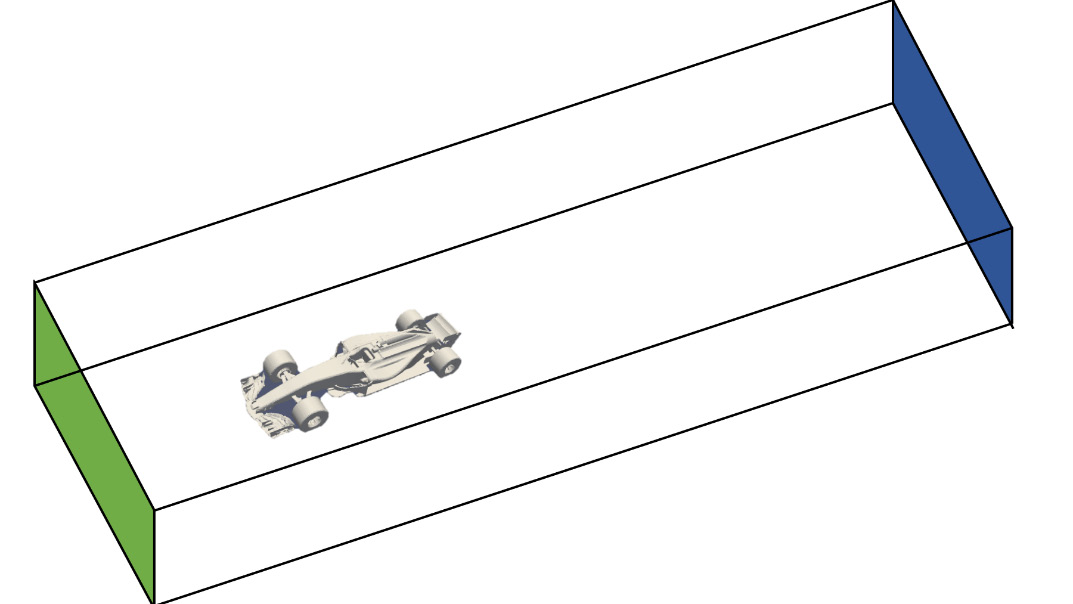
Figure 11.3 – CFD domain defined around the F1 car
The car and the domain so far are conceptual ideas and need to be represented as objects or files that CFD code can ingest and use. A typical file format used to represent objects is the Stereolithography (STL) file format. Each object is represented as a set of triangles, and each triangle is represented by a set of 3D points. The same car in an STL format is shown in Figure 11.4 – the car is now a collection of tens of thousands of triangles.

Figure 11.4 – F1 car in an STL format
We can now use this car object and mesh the CFD domain. Creating a mesh, or meshing, is the process of creating grid points in the CFD domain where numerical equations related to fluid flow are to be solved. Meshing is a very important process, as this can directly influence results, and also sometimes cause the numerical simulation to diverge or not solve.
Note
Meshing techniques and details about the algorithms used are beyond the scope of this book. Each solver tool implements different meshing techniques with various configurations. Teams spend a significant amount of time getting high-quality meshes while balancing the complexity of the mesh to ensure faster solving times.
Once the mesh is built out, it may look similar to Figure 11.5. We see that there is a concentration of grid cells closer to the body. Note that this is a slice of the mesh, and the actual mesh is a 3D volume with the bounds that were defined in Figure 11.3.

Figure 11.5 – CFD mesh built for the F1 car case
Once the mesh is built out, we can use CFD solvers to calculate the flow around this F1 car, and then post-process these results to provide us with predictions for drag and downforce. Figure 11.6 and Figure 11.7 show typical post-processed images involving streamlines (the white lines in the images representing how fluid flows around the body), a velocity slice (the magnitude of the velocity on a plane or cross-section of interest), pressure on the car body (redder regions are higher pressure), and the original car geometry for context.

Figure 11.6 – Post-processed results for the F1 car case showing streamlines and velocity slice
Figure 11.7 shows a different output visualization of pressure on the surface of the car, along with the streamlines in a perspective view.

Figure 11.7 – Post-processed results for the F1 car case showing pressure on the car body with streamlines
In summary, running a CFD case involves the following:
- Loading and manipulating the geometry
- Meshing the CFD domain
- Using a solver to solve for the flow in the domain
- Using post-processing tools to visualize the results
In the next section, we will discuss a few ways of running CFD analyses on AWS according to our documented best practices.
Reviewing best practices for running CFD on AWS
CFD, being very compute-intensive, needs to be scaled massively to be practical for companies that depend on analysis results to make decisions about their product designs. AWS allows customers to run CFD simulations at a massive scale (thousands of cores), on-demand, with multiple commercial and open source tools, and without any capacity planning or up-front capital investment. You can find many useful links related to CFD on AWS here: https://aws.amazon.com/hpc/cfd/.
As highlighted at the outset of this chapter, there are several commercial and open source tools available to solve your CFD problems that run at scale on AWS. Some of these tools are as follows:
- Siemens SimCenter STAR-CCM+
- Ansys Fluent
- OpenFOAM (open source)
In this chapter, we will be providing you with examples of how to set up and use OpenFOAM. For other tools, please take a look at this workshop provided by AWS: https://cfd-on-pcluster.workshop.aws/.
Note
Note that the AWS Well-Architected pillar defines best practices for running any kind of workload on AWS. It includes the best practices for designing architectures on AWS with the following pillars: Operational Excellence, Security, Reliability, Performance Efficiency, Cost Optimization, and Sustainability.
If you are unfamiliar with the Well-Architected Framework, you can read about it in detail here: https://docs.aws.amazon.com/wellarchitected/latest/framework/welcome.html/.
We will now discuss two different ways of running CFD simulations on AWS: using ParallelCluster and using CFD Direct.
Using AWS ParallelCluster
On AWS, these Well-Architected best practices are encapsulated in a solution called AWS ParallelCluster that you can launch in your AWS account. ParallelCluster lets you configure and launch an entire HPC cluster with a simple Command-Line Interface (CLI). The CLI also allows you to dynamically scale resources needed for your CFD (and other HPC) applications as needed, in a secure manner. Popular schedulers such as AWS Batch or Slurm can be used to submit and monitor jobs on ParallelCluster. Here are some steps to follow for installing ParallelCluster (note that a complete set of steps can be found on the official AWS documentation page for ParallelCluster here: https://docs.aws.amazon.com/parallelcluster/latest/ug/install-v3-pip.html).
Step 1 – creating an AWS Cloud9 IDE
This helps us have access to a full IDE on the cloud on a specified instance type, with temporary, managed credentials that can be used to launch ParallelCluster. Follow the instructions here to launch an AWS Cloud9 IDE: https://docs.aws.amazon.com/cloud9/latest/user-guide/setup-express.html.
Once you have created your Cloud9 IDE, navigate to the terminal as shown in the instructions here: https://docs.aws.amazon.com/cloud9/latest/user-guide/tour-ide.html#tour-ide-terminal.
Step 2 – installing the ParallelCluster CLI
Once you are inside the terminal, do the following:
- Use pip to install ParallelCluster:
...
python3 -m pip install "aws-parallelcluster" --upgrade –-user
...
- Next, make sure that you have Node Version Manager (NVM) installed:
...
curl -o- https://raw.githubusercontent.com/nvm-sh/nvm/v0.38.0/install.sh | bash
chmod ug+x ~/.nvm/nvm.sh
source ~/.nvm/nvm.sh
nvm install --lts
node –version
...
- Lastly, verify that ParallelCluster has been installed successfully:
pcluster version
{"version": "3.1.3"
}
Let’s move on to step 3.
Step 3 – configuring your ParallelCluster
Before you launch ParallelCluster, you need to define parameters using the configure command:
...
pcluster configure
...
The command-line tool will ask you the following questions for creating a configuration (or config, for short) file:
- Region in which to set up ParallelCluster (for example, US-East-1)
- EC2 Key Pair to use (learn more about Key Pairs here: https://docs.aws.amazon.com/AWSEC2/latest/UserGuide/ec2-key-pairs.html
- Operating system (for example, Amazon Linux 2, CentOS 7, or Ubuntu)
- Head node instance type (for example, c5n.18xlarge)
- Whether to automate VPC creation
- Subnet configuration (for example, head or main node placed in a public subnet with the rest of the compute fleet in a private subnet or subnets)
- Additional shared storage volume (for example, FSx configuration)
This creates a config file that can be found in ~/.parallelcluster and modified before the creation of the cluster. Here is an example of a ParallelCluster config file:
...
Region: us-east-2
Image:
  Os: alinux2
HeadNode:
  InstanceType: c5.4xlarge
  Networking:
    SubnetId: subnet-0e6e79abb7ed2452c
  Ssh:
    KeyName: pcluster
Scheduling:
  Scheduler: slurm
  SlurmQueues:
  - Name: queue1
    ComputeResources:
    - Name: c54xlarge
      InstanceType: c5.4xlarge
      MinCount: 0
      MaxCount: 4
    - Name: m516xlarge
      InstanceType: m5.16xlarge
      MinCount: 0
      MaxCount: 2
    Networking:
      SubnetIds:
      - subnet-09299f6d9ecfb8122
...
A deeper dive into the intricacies of the ParallelCluster config file can be found here: https://aws.amazon.com/blogs/hpc/deep-dive-into-the-aws-parallelcluster-3-configuration-file/.
Step 4 – launching your ParallelCluster
Once you have verified the config file, use the following command to create and launch ParallelCluster:
...
pcluster create-cluster --cluster-name mycluster --cluster-configuration config
{
  "cluster": {
    "clusterName": "mycluster",
    "cloudformationStackStatus": "CREATE_IN_PROGRESS",
    "cloudformationStackArn": "arn:aws:cloudformation:us-east-2:989279443319:stack/mycluster/c6fdb600-d49e-11ec-9c26-069b96033f9a",
    "region": "us-east-2",
    "version": "3.1.3",
    "clusterStatus": "CREATE_IN_PROGRESS"
  }
}...
Here, our cluster has been named mycluster. This will launch a CloudFormation template with the required resources to work with ParallelCluster, based on the config file you previously defined. The following services are used by AWS ParallelCluster:
- AWS Batch
- AWS CloudFormation
- Amazon CloudWatch
- Amazon CloudWatch Logs
- AWS CodeBuild
- Amazon DynamoDB
- Amazon Elastic Block Store
- Amazon Elastic Compute Cloud (EC2)
- Amazon Elastic Container Registry
- Amazon Elastic File System (EFS)
- Amazon FSx for Lustre
- AWS Identity and Access Management
- AWS Lambda
- NICE DCV
- Amazon Route 53
- Amazon Simple Storage Service
- Amazon VPC
For more details on the services used, please refer to the links provided in the References section of this chapter. A simplified architecture diagram of AWS ParallelCluster is shown in Figure 11.8 – more details can be found on the following blog: https://aws.amazon.com/blogs/compute/running-simcenter-star-ccm-on-aws/. Otherwise, see the documentation page for ParallelCluster (https://docs.aws.amazon.com/parallelcluster/latest/ug/what-is-aws-parallelcluster.html).

Figure 11.8 – AWS ParallelCluster architecture
The launch will typically take about 10 minutes and can be tracked both on the console as well as on the CloudFormation page on the AWS Management Console. On the console, the following message will confirm that your launch is in progress:
pcluster list-clusters --query 'clusters[?clusterName==`mycluster`]'
[
  {
    "clusterName": "mycluster",
    "cloudformationStackStatus": "CREATE_IN_PROGRESS",
    "cloudformationStackArn": "arn:aws:cloudformation:us-east-2:<account_number>:stack/mycluster/c6fdb600-d49e-11ec-9c26-069b96033f9a",
    "region": "us-east-2",
    "version": "3.1.3",
    "clusterStatus": "CREATE_IN_PROGRESS"
  }
]
Wait for the status to say "clusterStatus": "CREATE_COMPLETE"
Step 5 – installing OpenFOAM on the cluster
To install OpenFOAM on your cluster, see the following:
- First, add Secure Shell (SSH) into the head node of your newly created ParallelCluster:
pcluster ssh -n mycluster -i pcluster.pem
The authenticity of host '3.135.195.149 (3.135.195.149)' can't be established.
ECDSA key fingerprint is SHA256:DZPeIcVRpZDg3VMYhA+2zAvEoLnD3gI6mLVkMPkyg90.
ECDSA key fingerprint is MD5:87:16:df:e7:26:f5:a0:da:a8:3a:7c:c4:c8:92:60:34.
Are you sure you want to continue connecting (yes/no)? yes
Warning: Permanently added '3.135.195.149' (ECDSA) to the list of known hosts.
Last login: Sun May 15 22:36:41 2022
__| __|_ )
_| ( / Amazon Linux 2 AMI
___|\___|___|
- You are now in the head node of the ParallelCluster. Next, download the OpenFOAM files as follows:
...
wget https://sourceforge.net/projects/openfoam/files/v2012/OpenFOAM-v2012.tgz
wget https://sourceforge.net/projects/openfoam/files/v2012/ThirdParty-v2012.tgz
...
- Next, untar the two files you just downloaded:
...
tar -xf OpenFOAM-v2012.tgz
tar -xf ThirdParty-v2012.tgz
...
- Change the directory to the newly extracted OpenFOAM folder and compile OpenFOAM:
...
cd OpenFOAM-v2012
export WM_NCOMPPROCS=36
./Allwmake
...
To install OpenFOAM on all nodes, you can use the sbatch command, and submit the preceding commands as a file named compile.sh: for example, sbatch compile.sh.
Once installation completes, you can run a sample CFD application as shown in step 6.
Step 6 – running a sample CFD application
Here, we will run a sample CFD application using ParallelCluster. First, we access the head node of the cluster we just created using SSH:
...
pcluster ssh --cluster-name mycluster -i /path/to/keyfile.pem
...
Make sure you use the same .pem file that you created in step 3!
In this case, we will be running an example from OpenFOAM – incompressible flow over a motorbike. The case files for this case can be found here: https://static.us-east-1.prod.workshops.aws/public/a536ee90-eecd-4851-9b43-e7977e3a5929/static/motorBikeDemo.tgz.
The geometry corresponding to this case is shown in Figure 11.9.

Figure 11.9 – Geometry for the motorbike case in OpenFOAM
To run the case in just the head node, you can run the following commands:
cp $FOAM_TUTORIALS/resources/geometry/motorBike.obj.gz constant/triSurface/
surfaceFeatureExtract
blockMesh
snappyHexMesh
checkMesh
potentialFoam
simpleFoam
We will go into detail about what these commands do in later sections. For now, our aim is just to run the example motorbike case.
To run the same case in parallel with all your compute nodes, you can use sbatch to submit the following shell script (similar to submitting the installation shell script). We can define some input arguments to the script, followed by loading OpenMPI and OpenFOAM:
...
#!/bin/bash
#SBATCH --job-name=foam
#SBATCH --ntasks=108
#SBATCH --output=%x_%j.out
#SBATCH --partition=compute
#SBATCH --constraint=c5.4xlarge
module load openmpi
source OpenFOAM-v2012/etc/bashrc
cp $FOAM_TUTORIALS/resources/geometry/motorBike.obj.gz constant/triSurface/
First, we mesh the geometry using the blockMesh and snappyHexMesh tools (see the following code):
surfaceFeatureExtract  > ./log/surfaceFeatureExtract.log 2>&1
blockMesh  > ./log/blockMesh.log 2>&1
decomposePar -decomposeParDict system/decomposeParDict.hierarchical  > ./log/decomposePar.log 2>&1
mpirun -np $SLURM_NTASKS snappyHexMesh -parallel -overwrite -decomposeParDict system/decomposeParDict.hierarchical   > ./log/snappyHexMesh.log 2>&1
We then check the quality of the mesh using checkMesh, and renumber and print out a summary of the mesh (see code):
mpirun -np $SLURM_NTASKS checkMesh -parallel -allGeometry -constant -allTopology -decomposeParDict system/decomposeParDict.hierarchical > ./log/checkMesh.log 2>&1
mpirun -np $SLURM_NTASKS redistributePar -parallel -overwrite -decomposeParDict system/decomposeParDict.ptscotch > ./log/decomposePar2.log 2>&1
mpirun -np $SLURM_NTASKS renumberMesh -parallel -overwrite -constant -decomposeParDict system/decomposeParDict.ptscotch > ./log/renumberMesh.log 2>&1
mpirun -np $SLURM_NTASKS patchSummary -parallel -decomposeParDict system/decomposeParDict.ptscotch > ./log/patchSummary.log 2>&1
ls -d processor* | xargs -i rm -rf ./{}/0
ls -d processor* | xargs -i cp -r 0.orig ./{}/0
Finally, we run OpenFOAM through the potentialFoam and simpleFoam binaries as shown here:
mpirun -np $SLURM_NTASKS potentialFoam -parallel -noFunctionObjects -initialiseUBCs -decomposeParDict system/decomposeParDict.ptscotch > ./log/potentialFoam.log 2>&1s
mpirun -np $SLURM_NTASKS simpleFoam -parallel  -decomposeParDict system/decomposeParDict.ptscotch > ./log/simpleFoam.log 2>&1
...
You can follow instructions in the following AWS workshop to visualize results from the CFD case: https://catalog.us-east-1.prod.workshops.aws/workshops/21c996a7-8ec9-42a5-9fd6-00949d151bc2/en-US/openfoam/openfoam-visualization.
Let’s discuss CFD Direct next.
Using CFD Direct
In the previous section, we saw how you can run a CFD simulation using ParallelCluster on AWS. Now, we will look at how to run CFD using the CFD Direct offering on AWS Marketplace: https://aws.amazon.com/marketplace/pp/prodview-ojxm4wfrodtj4. CFD Direct provides an Amazon EC2 image built on top of Ubuntu with all the typical tools you need to run CFD with OpenFOAM.
Perform the following steps to get started:
- Follow the link above to CFD Direct’s Marketplace offering, and click Continue to Subscribe.
- Then, follow the instructions provided and click Continue to Configure (leave all options as the default), and then Continue to Launch. Similar to ParallelCluster, remember to use the right EC2 key pair so you can SSH into the instance that is launched for you.

Figure 11.10 – CFD Direct AWS Marketplace offering (screenshot taken as of August 5, 2022)
Follow the instructions and get more help on using CFD Direct’s image here: https://cfd.direct/cloud/aws/.
To connect to the instance for the first time, use the instructions given here: https://cfd.direct/cloud/aws/connect/.
In the following tutorial, we will use the NICE DCV client as a remote desktop to interact with the EC2 instance.
To install NICE DCV, perform the following steps:
- First, SSH into the instance you just launched, and then download and install the server. For example, with Ubuntu 20.04, use the following command:
wget https://d1uj6qtbmh3dt5.cloudfront.net/nice-dcv-ubuntu2004-x86_64.tgz
- Then, execute the following command to extract the tar file:
tar -xvzf nice-dcv-2022.0-12123-ubuntu2004-x86_64.tgz && cd nice-dcv-2022.0-12123-ubuntu2004-x86_64
- Install NICE DCV by executing the following:
sudo apt install ./nice-dcv-server_2022.0.12123-1_amd64.ubuntu2004.deb
- To start the NICE DCV server, use the following command:
sudo systemctl start dcvserver
- Finally, start a session using the following:
dcv create-session cfd
- Find the public IP of your launched EC2 instance and use any NICE DCV client to connect to the instance (see Figure 11.11):

Figure 11.11 – Connecting to the EC2 instance using a public IP
- Next, use the username and password for Ubuntu (see Figure 11.12). If you haven’t set a password, use the passwd command on a terminal using SSH.

Figure 11.12 – Entering a username and password for Ubuntu
- If prompted, select the session you want to connect to. Here, we started a session called cfd. You should now be looking at your Ubuntu desktop with OpenFOAM 9 preinstalled.

Figure 11.13 – Ubuntu desktop provided by CFD Direct
- To locate all the OpenFOAM tutorials to try out, use the following command:
echo $FOAM_TUTORIALS
/opt/openfoam9/tutorials
- We will run a basic airfoil tutorial that is located in the following directory:
/opt/openfoam9/tutorials/incompressible/simpleFoam/airFoil2D/
The directory is set up like a typical OpenFOAM case and has the following contents (explore using the tree command on Ubuntu):
/opt/openfoam9/tutorials/incompressible/simpleFoam/airFoil2D/
|-- 0
|   |-- U
|   |-- nuTilda
|   |-- nut
|   `-- p
|-- Allclean
|-- Allrun
|-- constant
|   |-- momentumTransport
|   |-- polyMesh
|   |   |-- boundary
|   |   |-- cells
|   |   |-- faces
|   |   |-- neighbour
|   |   |-- owner
|   |   `-- points
|   `-- transportProperties
`-- system
    |-- controlDict
    |-- fvSchemes
    `-- fvSolution
Let us explore some of these files, as this will give you an understanding of any OpenFOAM case. The folder called 0 represents the initial conditions (as in, time step 0) for these key quantities we will be solving for:
- Velocity (U)
- Pressure (p)
What do these files look like? Let’s take a look at the U (velocity) file:
FoamFile
{
    format      ascii;
    class       volVectorField;
    object      U;
}
dimensions      [0 1 -1 0 0 0 0];
internalField   uniform (25.75 3.62 0);
boundaryField
{
    inlet
    {
        type            freestreamVelocity;
        freestreamValue $internalField;
    }
    outlet
    {
        type            freestreamVelocity;
        freestreamValue $internalField;
    }
    walls
    {
        type            noSlip;
    }
    frontAndBack
    {
        type            empty;
    }
}
As we can see here, the file defines the dimensions of the CFD domain and the free stream velocity, along with the inlet, outlet, and wall boundary conditions.
The Airfoil2D folder also contains a folder called constant; this folder contains files specific to the CFD mesh that we will be creating. The momentumTransport file defines the kind of models to be used to solve this problem:
simulationType RAS;
RAS
{
    model           SpalartAllmaras;
    turbulence      on;
    printCoeffs     on;
}
Here, we use the SpalartAllmaras turbulence model under the Reynolds-Averaged Flow (RAF) type. For more information about this, please visit https://www.openfoam.com/documentation/guides/latest/doc/guide-turbulence-ras-spalart-allmaras.html.
The boundary file inside the polyMesh folder contains definitions of the walls themselves; this is to let the simulation know what a surface inlet or wall represents. There are several other files in the polyMesh folder that we will not explore in this section.
Inside the System folder, the controlDict file defines what applications to run for this case. OpenFOAM contains over 200 compiled applications; many of these are solvers and preprocessing and post-processing for the code.
Finally, we get to one of the most important files you will find in any OpenFOAM case: the Allrun executable. The Allrun file is a shell script that runs the steps we defined earlier for every typical CFD application in order – to import the geometry, create a mesh, solve the CFD problem, and post-process results.
Depending on the output intervals defined in your ControlDict file, several output folders will be output in the same directory that correspond to different time stamps in the simulation. The CFD solvers will solve the problem until they converge, or until a maximum number of time steps is reached. The output folders will look similar to the timestep 0 folder that we created earlier. To visualize these results, we use a tool called ParaView:
- First, let us look at the mesh we have created (see Figure 11.14). The executables included within OpenFOAM that are responsible for creating this mesh are blockmesh and snappyhexmesh. You can also run these commands manually instead of running the Allrun file.

Figure 11.14 – Mesh for the Airfoil 2D case in OpenFOAM
- Great – after solving the problem using the SimpleFoam executable, let us take a look at the pressure distribution around the airfoil (see Figure 11.15):

Figure 11.15 – Pressure distribution for the Airfoil 2D case in OpenFOAM
- Lastly, we can use ParaView to visualize the velocity distribution, along with streamlines (see Figure 11.16):

Figure 11.16 – Velocity distribution for the Airfoil 2D case in OpenFOAM
Note that these plots are post-processed by initializing ParaView with the paraFoam executable, which automatically understands output formatted by OpenFOAM cases.
Let us now look at a slightly more complicated case – the flow around a car:
- First, let us look at the geometry of the car (Figure 11.17 and Figure 11.18):

Figure 11.17 – Car geometry (perspective view)

Figure 11.18 – Car geometry (side view)
- Next, we can use the blockmesh and snappyhexmesh commands to create the CFD mesh around this car (see Figure 11.19):
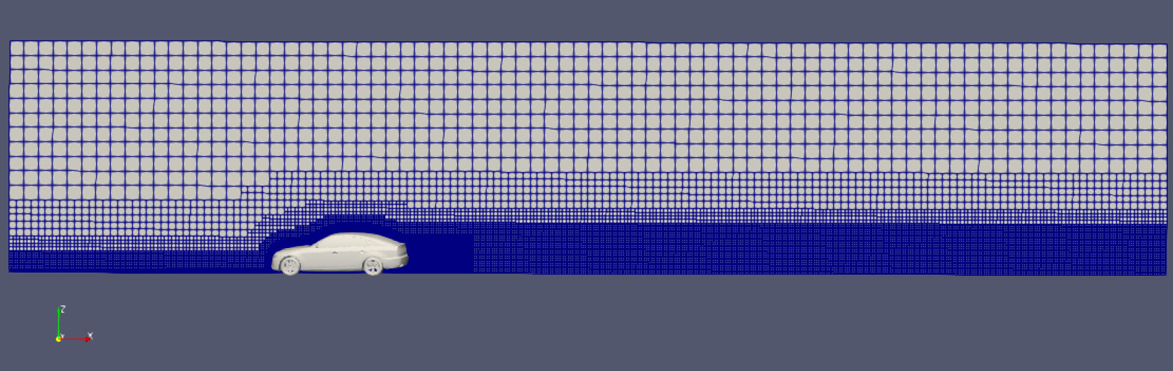
Figure 11.19 – Mesh created for the car case
- We can then run the Allrun file to solve the problem. Finally, we will visualize the output (Figures 11.20 and Figure 11.21):

Figure 11.20 – Streamlines (black) and pressure distribution (perspective view) created for the car case
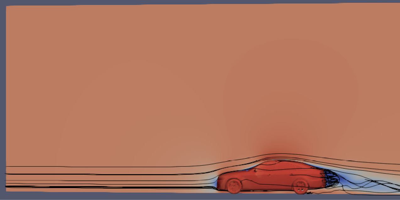
Figure 11.21 – Streamlines (black) and pressure distribution (side view) created for the car case
The files needed for the following cases can be found in the ZIP files provided in the GitHub repository here: https://github.com/PacktPublishing/Applied-Machine-Learning-and-High-Performance-Computing-on-AWS/tree/main/Chapter11/runs.
In the next section, we will discuss some advancements in the CFD field related to using ML and deep learning with CFD tools.
Discussing how ML can be applied to CFD
CFD, being a field that has been around for decades, has matured to be very useful to companies in various domains and has also been implemented at scale using cloud providers. Recent advances in ML have been applied to CFD, and in this section, we will provide readers with pointers to articles written about this domain.
Overall, we see deep learning techniques being applied in two primary ways:
- Using deep learning to map inputs to outputs. We explored the flow over an airfoil in this chapter and visualized these results. If we had enough input variation and saved the outputs as images, we could use autoencoders or Generative Adversarial Networks (GANs) to generate these images. As an example, the following paper uses GANs to predict flows over airfoils using sparse data: https://www.sciencedirect.com/science/article/pii/S1000936121000728. As we can see in Figure 11.22, the flow fields predicted by CFD and the GAN are visually very similar:

Figure 11.22 – Pressure distribution generated by a trained GAN (left) and CFD (right)
Similarly, Autodesk trained a network with over 800 examples of cars and can instantaneously predict the flow and drag of a new car body: https://dl.acm.org/doi/10.1145/3197517.3201325 (see figure 11.23).

Figure 11.23 – Flow field and drag coefficient being predicted instantaneously for various car shapes
- The second general type of innovation is not just mapping inputs to outputs, but actually using ML techniques as part of the CFD solver itself. For example, NVIDIA’s SIMNET (https://arxiv.org/abs/2012.07938) paper describes how deep learning can be used to model the actual Partial Differential Equations (PDEs) that define the fluid flow and other physical phenomena. See Figure 11.24 for example results from SIMNET for flow over a heat sink. Parameterized training runs are faster than commercial and open source solvers, and inference for new geometries are instantaneous.

Figure 11.24 – Velocity (top row) and temperature (bottom row) comparisons of OpenFOAM versus SIMNET from NVIDIA
Let’s summarize what you have learned in this chapter next.
Summary
In this chapter, we provided a high-level introduction to the world of CFD, and then explored multiple ways to use AWS to solve CFD problems (using ParallelCluster and CFD Direct on EC2). Finally, we discussed some recent advancements connecting the field of CFD to ML. While it is out of the scope of this book to go into much more detail regarding CFD, we hope that the readers are inspired to dive deeper into the topics explored here.
In the next chapter, we will focus on genomics applications using HPC. Specifically, we will talk about drug discovery and do a detailed walk-through of a protein structure prediction problem.
References
- AWS Batch: https://docs.aws.amazon.com/parallelcluster/latest/ug/aws-services-v3.html#aws-batch-v3
- AWS CloudFormation: https://docs.aws.amazon.com/parallelcluster/latest/ug/aws-services-v3.html#aws-services-cloudformation-v3
- Amazon CloudWatch: https://docs.aws.amazon.com/parallelcluster/latest/ug/aws-services-v3.html#amazon-cloudwatch-v3
- Amazon CloudWatch Logs: https://docs.aws.amazon.com/parallelcluster/latest/ug/aws-services-v3.html#amazon-cloudwatch-logs-v3
- AWS CodeBuild: https://docs.aws.amazon.com/parallelcluster/latest/ug/aws-services-v3.html#aws-codebuild-v3
- Amazon DynamoDB: https://docs.aws.amazon.com/parallelcluster/latest/ug/aws-services-v3.html#amazon-dynamodb-v3
- Amazon Elastic Block Store: https://docs.aws.amazon.com/parallelcluster/latest/ug/aws-services-v3.html#amazon-elastic-block-store-ebs-v3
- Amazon Elastic Container Registry: https://docs.aws.amazon.com/parallelcluster/latest/ug/aws-services-v3.html#amazon-elastic-container-registry-ecr-v3
- Amazon EFS: https://docs.aws.amazon.com/parallelcluster/latest/ug/aws-services-v3.html#amazon-efs-v3
- Amazon FSx for Lustre: https://docs.aws.amazon.com/parallelcluster/latest/ug/aws-services-v3.html#amazon-fsx-for-lustre-v3