Chapter 2: How Does CockroachDB Work Internally?

In the previous chapter, we learned about the evolution of databases and the high-level architecture of CockroachDB. In this chapter, we will go a bit deeper into each of the layers of CockroachDB and explore how CockroachDB works internally. We will also discuss some of the core design aspects that form the basic pillars of CockroachDB.

CockroachDB can be broadly divided into five main layers, as outlined here:

• Structured Query Language (SQL)
• Transactional
• Distribution
• Replication
• Storage

Each of these layers will be explained as the main topics of this chapter, in the following order:

• Installing a single-node CockroachDB cluster using Docker
• Execution of a SQL query
• Managing a transactional key-value store
• Data distribution across multiple nodes
• Data replication for resilience and availability
• Interactions with the disk for data storage

Since we will be trying out some commands in this chapter, it's important to have a working environment for them. So, we will start with the technical requirements, where we will go over how to set up a single-node CockroachDB cluster.

Technical requirements

To try out some of the commands in this chapter, you will need a single-node CockroachDB cluster. There are several ways of installing CockroachDB on a computer, as outlined here:

• Use a package manager such as Homebrew to install it, but this option only works on a Mac.
• Download binaries, extract it, and set it in the PATH variable.
• Use Kubernetes to orchestrate CockroachDB pods.
• Build from source and install.
• Download a Docker image and run it.

In the current chapter, we will just go over how to run CockroachDB using Docker since the steps are common, irrespective of the operating system that you are using.

To use CockroachDB with Docker, you need a computer with the following:

• At least 4 gigabytes (GB) of random-access memory (RAM)
• 250 GB of disk space
• Docker installed

In the next section, we will learn about installing CockroachDB.

Installing a single-node CockroachDB cluster using Docker

Let's take a look at how to install a single-node CockroachDB cluster, which will be required to try out some of the commands that will be introduced in this chapter. Here are the steps you need to follow:

1. Ensure the Docker daemon is running with the following command:

   docker version

Pull the most recent stable version with tag v<xx.y.z> from https://hub.docker.com/r/cockroachdb/cockroach/. Take a look at the following example:

docker pull cockroachdb/cockroach:v20.2.4

2. Make sure this image is available and the version is correct with the help of the following command:

   docker images | grep cockroach

   cockroachdb/cockroach   v20.2.4             d47481b0b677        2 days ago          329MB

If running docker on windows, then replace grep with findstr:

docker images | findstr cockroach

3. Create a bridge network. A bridge network allows multiple containers to communicate with each other. Here's the code you'll need to create one:

   $ docker network create -d bridge crdb_net

4. Create a volume. Volumes are used for persisting data generated and used by Docker containers. Since CockroachDB is a database, it needs a place to store the data, and hence we should attach a volume to the container. You can do this by running the following command:

   $ docker volume create crdb_vol1

5. Start a CockroachDB node using the following command:

   $ docker run -d

   --name=crdb1

   --hostname=crdb1

   --net=crdb_net

   -p 26257:26257 -p 8080:8080  

   -v "crdb_vol1:/cockroach/cockroach-data"  

   cockroachdb/cockroach:v20.2.4 start

   --insecure

   --join=crdb_vol1

   • Here is an explanation of what each of these options means:
   • docker run: This starts a Docker container.
   • --name: Name of the container.
   • --hostname: Hostname of the container. This will be useful if you are running multiple containers and want to join them to form a cluster.
   • --net: Bridge network. This will be useful if you have more than one container that wants to communicate with other containers.
   • -p 26257:26257: Port mapping for inter-node or SQL client for node communication.
   • -p 8080:8080: Port mapping used for HyperText Transfer Protocol (HTTP) requests to the CockroachDB console.
   • -v "crdb_vol1:/cockroach/cockroach-data": Mounts the host directory as a data volume.
   • cockroachdb/cockroach:v20.2.4 start: Command to start the CockroachDB node.
   • --insecure: Option to start the node in insecure mode.
   • --join=crdb_vol1: Here, you can specify multiple hostnames of CockroachDB nodes that will form a cluster. For the current chapter, we just need a single-node cluster.
6. Initialize the cluster with the following command:

   $ docker exec -it crdb1 ./cockroach init --insecure

   Cluster successfully initialized

7. To ensure that the CockroachDB node is functional, we can create a database and a table, insert some data, and run a query.

The following command is used for starting the SQL shell:

docker exec -it crdb1 ./cockroach sql -–insecure

The following command is used for creating a database:

root@:26257/defaultdb> CREATE DATABASE testdb;

The following command is used for creating a table:

root@:26257/defaultdb> CREATE TABLE testdb.testtable (id INT PRIMARY KEY, string name);

8. Verify the columns by running the following code:

   root@:26257/defaultdb> SHOW COLUMNS from testdb.testtable;

     column_name | data_type | is_nullable | column_default | generation_expression |  indices  | is_hidden

   --------------+-----------+-------------+----------------+-----------------------+-----------+------------

     id          | INT8      |    false    | NULL           |                       | {primary} |   false

     string      | NAME      |    true     | NULL           |                       | {}        |   false

   (2 rows)

   Time: 134ms total (execution 133ms / network 1ms)

9. Insert some data, as follows:

   root@:26257/defaultdb> INSERT INTO testdb.testtable VALUES (1,'Spencer Kimball'), (2,'Ben Darnell'), (3,'Peter Mattis');

Run a query to fetch the contents of the table:

root@:26257/defaultdb> SELECT * FROM testdb.testtable;

  id |     string

-----+------------------

   1 | Spencer Kimball

   2 | Ben Darnell

   3 | Peter Mattis

(3 rows)

Time: 5ms total (execution 3ms / network 2ms)

Next, we will learn about each of the layers, starting with the SQL layer.

Execution of a SQL query

Any application that talks to CockroachDB can use Postgres-compatible drivers to talk to CockroachDB. If you prefer object-relational mappers (ORMs), Golang ORM (GORM), go-pg, and SQLBoiler can be used to interact with CockroachDB. Irrespective of where the actual data resides, you can issue a query to any of the nodes in the cluster. Whichever node the query lands in, that node acts as a gateway.

Requests from SQL clients are received as SQL statements. The SQL layer is responsible for converting these SQL statements into a plan of key-value operations and passing it to the transaction layer. CockroachDB, as of version 21.2, supports both native drivers and the Postgres wire protocol. A wire protocol defines how two applications can communicate over a network.

CockroachDB has support for most American National Standards Institute (ANSI) SQL standards to change table structures and data. Next, we will look at the various stages of query execution.

SQL query execution

As with any other database, there are standard steps involved in processing incoming SQL requests and serving the data.

Before going through the different steps of a SQL layer, it's important to get ourselves familiar with some terms related to SQL, as follows:

• An SQL parser is software that scans a given SQL statement in its string form and tries to make sense of it. This involves lexical analysis, which is extracting the tokens or the keywords, and syntactic analysis, where you make sure the entire query is valid and can be represented in a form that makes it easier to execute the query. Lex is a popular lexical analyzer and Yacc (which stands for Yet Another Compiler-Compiler) is software that processes grammar and generates a parser.
• An abstract syntax tree (AST) or a syntax tree is a tree representation of a given domain-specific language. Nodes in the tree represent constructs in that language. ASTs are essential for deciding on how to execute a given query.

Some of the main steps in a SQL layer include query parsing, logical planning, physical planning, and query execution. Vectorized query execution is enabled by default, which gives much better performance.

Parsing

CockroachDB uses Goyacc, Golang's equivalent of the famous C Yacc to generate a SQL parser from a grammar file located at pkg/sql/parser/sql.y. This parser then converts the input into an AST comprising of tree nodes, where the node types are defined under the pkg/sql/sem/tree package.

Logical planning

Once we have an AST, it then has to be transformed into a logical plan. A logical plan defines how various clauses can be logically ordered. As part of this transformation, semantic analysis is initially done for type checking, name resolution, and to ensure the query is valid. Later, this logic plan is simplified without changing the overall semantics and is optimized based on the cost. Here, cost refers to the total time taken to return the results of a query. Cost optimization involves picking the right indexes, query optimization, and selecting the best strategies for sorting and joining. We can view the logical plan using EXPLAIN <SQL Statement>.

The following example shows the output of a sample EXPLAIN query:

root@:26257/defaultdb> EXPLAIN SELECT * FROM testdb.testtable;

  tree |        field        |    description

-------+---------------------+--------------------

       | distribution        | full

       | vectorized          | false

  scan |                     |

       | estimated row count | 1

       | table               | testtable@primary

       | spans               | FULL SCAN

(6 rows)

Time: 11ms total (execution 10ms / network 1ms)

Physical planning

In this phase, all the participating nodes are determined based on where the data resides and also who is the primary owner for a given range, which is also known as a range's leaseholder. Typically, partial result sets are gathered from various nodes that are then sent to the coordinator or the gateway node, which aggregates all the results and sends a single response back to the SQL client. Let's look at an example of what this looks like for a sample query for the testdb.testtable table that we created in step 8 in the Installing a single node CockroachDB cluster using Docker section.

Let's assume we have six names that are distributed across four nodes in a cluster. The following table shows information about the leaseholder nodes, key ranges, and user data:

Figure 2.1 – Table showing information about key ranges

Now, let's assume that a SQL client sends a query to fetch all the names from the testdb.testtable table. In this example, this request lands in node 1, so it acts as a gateway node that is responsible for collecting the data required to serve this request after coordinating with all relevant leaseholder nodes, getting a partial result, aggregating the data, and sending it back to the SQL client. This process is illustrated in the following screenshot:

Figure 2.2 – How a given query is served from the gateway node

At Gateway Node, the main challenge is to identify whether a given computation should be pushed down to nodes where the data resides or to do the same computation within the coordinator node on an aggregated result. The physical plan aims to make the best use of parallel computing and at the same time reduce the overall data that gets transferred between data and coordinator nodes. Also, table joins bring in an added layer of complexity. We can view the physical plan using EXPLAIN(DISTSQL) <SQL statement>. DISTSQL generates a Uniform Resource Locator (URL) for a physical query plan, which includes high-level information about how the query will be executed.

The following example shows the output of a sample EXPLAIN(DISTSQL) query:

root@:26257/defaultdb> EXPLAIN(DISTSQL) SELECT * FROM testdb.testtable where id > 1;

  automatic |                                               url

------------+---------------------------------------------------------------------------------------------------------------------------------------------------------------------------------------------------------------------------------------------------------------------------------------------------------------------------------------------------------------------------------------------------------

    false   | https://cockroachdb.github.io/distsqlplan/decode.html#eJyMj0FLxDAQhe_-ivBOKtFt9ZaTohULdXdtCwraQ7YZlkK3qZkUlNL_Lm1A8SDsKbz3Mu-bGcEfLRSS1212m67F6X1alMVzdiaKJEvuSnEuHvLNk_DE3uwu58frXUvi5THJE9EY8T5E0TWJGBKdNbTWB2KoN8SoJHpna2K2brbG5UNq PqEiiabrBz_blURtHUGN8I1vCQrljMhJG3KrCBKGvG7apfZng5veNQftviBR9LpjJVZXF6gmCTv432r2ek9Q8SSPx-fEve2Y_pD_a46mSoLMnsKJbAdX09bZesEEuVnmFsMQ-5DGQaRdiKZqOvkOAAD__6E0gSw=

(1 row)

Time: 21ms total (execution 16ms / network 4ms)

As you can see, the output is a downloadable URL for the actual physical plan. If you click on that URL, it will take you to the physical plan, as shown in the following screenshot:

Figure 2.3 – Visual representation of a physical plan in a single-node cluster

The EXPLAIN ANALYZE statement (https://www.cockroachlabs.com/docs/v21.1/sql-statements) executes a SQL query and generates a statement plan with execution statistics, as illustrated in the following code snippet:

root@:26257/testdb> EXPLAIN ANALYZE SELECT * FROM testdb.testtable;

  automatic |                                               url

------------+-------------------------------------------------------------------------------------------------------------------------------------------------------------------------------------------------------------------------------------------------------------------------------------------------------------------------------------------------------------------------------------------------------------------------------------------------

    true    | https://cockroachdb.github.io/distsqlplan/decode .html#eJyMUE1L60AU3b9fMZzVe4-xNhZdzMqqEQKxrU0XfpDFNHMpgSQT596i peS_SxJUXAiuhvMx5xzuEfxSwSB-WKXzZKHmi3n6-BSrvzdJtsnu038qi9P4eq P-q9v18k4JsbjtpH_EbiuCRuMdLWxNDPOMCLlGG3xBzD701HEwJO4NZqpRNu1ee jrXKHwgmCOklIpgsOkD12QdhdMpNByJLash9rPvsg1lbcMBGllrGzbq BBrBv7IKZJ1RM2iw2KpSUtZkVDSZXcxqhsb2IPThis7O1RXyTsPv5WsRi90RTNT p369eE7e-Yfo2-KfkaZdrkNvReBn2-1DQKvhiqBnhcvg3EI5YRjUaQdKMUpd3f9 4DAAD__yWSjvw=

(1 row)

Time: 4ms total (execution 3ms / network 1ms)

The output is shown here:

Figure 2.4 – Statement plan with execution statistics

EXPLAIN ANALYZE (DEBUG) executes a query and generates a link to a ZIP file that contains the physical statement plan (https://www.cockroachlabs.com/docs/stable/explain-analyze.html#distsql-plan-viewer), execution statistics, statement tracing, and other information about the query. The code is illustrated in the following snippet:

root@:26257/testdb> EXPLAIN ANALYZE (DEBUG) SELECT * FROM testdb.testtable;

                                      text

--------------------------------------------------------------------------------

  Statement diagnostics bundle generated. Download from the Admin UI (Advanced

  Debug -> Statement Diagnostics History), via the direct link below, or using

  the command line.

  Admin UI: http://crdb1:8080

  Direct link: http://crdb1:8080/_admin/v1/stmtbundle/676836398188756993

  Command line: cockroach statement-diag list / download

(6 rows)

Time: 92ms total (execution 91ms / network 1ms)

Query execution

During query execution, the physical plan is pushed down to all the data nodes that would be involved in serving a given query. CockroachDB uses work units called logical processors, which will be responsible for executing relevant computations. Logical processors across data nodes also communicate with each other so that data can be sent back to the coordinator or the gateway node.

There are two types of query execution, as outlined here:

• Non-vectorized or row-oriented query execution
• Vectorized or column-oriented query execution

Vectorized query execution (column-oriented query execution) is more suited to analytical workloads, whereas non-vectorized query execution (row-oriented query execution) is preferred for transactional workloads. By default, vectorized query execution is enabled on CockroachDB.

Now, let's take a look at how CockroachDB provides a transactional key-value store.

Managing a transactional key-value store

A transactional layer involves implementing a concurrency control protocol, as multiple transactions can try to update the same data at the same time, which can result in a conflict. In concurrency control, there are two different ways of dealing with conflicts, as outlined here:

• Avoid conflicts altogether with pessimistic locking—for example, a read/write lock.
• Let the conflict happen but detect it with optimistic locking and resolve it—for example, multi-version concurrency control (MVCC).

CockroachDB uses MVCC. In MVCC, there can be multiple versions of the same record, but you resolve the conflicts before committing the changes.

In CockroachDB, a given transaction is executed in three phases, outlined next:

1. A transaction is started with a target range that will participate in the transaction. A new transaction record is created to track the status of the transaction. It will have the initial state as PENDING. At the same time, a write intent is created. In CockroachDB, instead of directly writing the data to the storage layer, data is written to a provisional state called write intent. Here, the intent flag indicates that the value will be committed once the transaction is committed. CockroachDB uses MVCC for concurrency control. The transaction identifier (ID) is used to resolve conflicts for write intents. Each node involved in the transaction returns the timestamp used for the write, and the coordinator node selects the highest timestamp among all write timestamps and uses it in the final commit timestamp.
2. The transaction is marked as committed by updating its transaction record. The commit value also contains the candidate timestamp. The candidate timestamp is a temporary timestamp to denote when the transaction is committed and is selected as the actual node coordinating the transaction. Once the transaction is completed, control is returned to the client.
3. After the transaction is committed, all written intents are updated in parallel by removing the intent flag. The transaction coordinator does not wait for this step to be completed before returning the control to the client.

We will learn more about conflict resolution, atomicity, consistency, isolation, and durability (ACID), logical clocks, and transaction management in the next chapter. Next, we will go over the distributed layer.

Data distribution across multiple nodes

A table in CockroachDB can be partitioned, and this is discussed in Chapter 4, Geo-Partitioning, where we talk about geo-partitioning. CockroachDB stores the data in a monolithic sorted key-value store (MSKVS). Key-space is all the data you have in a given cluster, including information about its location. Key-space is divided into contiguous batches, called ranges. The MSKVS makes it easy to access any data from any node, which makes it possible for any node in the cluster to act as a gateway node, coordinating one or more data nodes while serving client requests.

The MSKVS

The MSKVS contains two categories of data, as outlined here:

• System data, which contains meta ranges, where the data of each range can be found within the cluster.
• User data, which is the actual table data.

Meta ranges

The location of ranges is maintained in two-level indexes, known as meta ranges. The first level (a.k.a. meta1) points to the second level (a.k.a. meta2) and the second-level indexes point to the actual data. This is shown in the following screenshot:

Figure 2.5 – Meta-range management in two levels

Every node in the cluster has complete information of meta1 and that range is never split. meta2 data is cached on nodes. These are invalidated whenever ranges change, and the cache gets updated with the latest value.

Let's look at an example.

Here, we will understand what meta1 and meta2 data looks like for an alphabetically sorted column. When we write ranges, square brackets '[' and ']' indicate that the number is included in the range, and parentheses '(' and ')' mean that the number is excluded.

Let's look at some examples here:

• [1,10]—range starts from 1 and ends at 10 as both numbers are included
• [1,5)—range starts from 1 and ends at 4, as 5 is excluded
• (1, 8)—range starts from 2, as 1 is excluded and it ends at 7, as 8 is excluded

Let's now understand what meta1 and meta2 look like for an alphabetically sorted column, as follows:

1. meta1 contains addresses of nodes that contain meta2 replicas. Let's assume there are two meta1 entries for simplicity.

The first meta1 entry points to the meta2 range for keys [A-M), and the second meta1 entry points to the meta2 range for keys [M-Z]. Here, maxKey indicates the rest of the range till the maximum available key. Since we are talking about an alphabetically sorted column, that would start at M, as the previous range excluded M and ends at Z, which is the last letter of the alphabet. The code is illustrated here:

meta1/M -> node1:26257, node2:26257, node3:26257

meta1/maxKey -> node4:26257, node5:26257, node6:26257

2. meta2 contains addresses of the nodes containing actual user data for that alphabetically sorted column. The first entry in the value always refers to the leaseholder, which is the primary owner of a given range. The code is illustrated here:

   meta2 entry for the range [A-G)

   meta2/G -> node1:26257, node2:26257, node3:26257

   meta2 entry for the range [G-M)

   meta2/M -> node1:26257, node2:26257, node3:26257

   meta2 entry for the range [M-Z)

   meta2/Z -> node4:26257, node5:26257, node6:26257

   meta2 entry for the range [Z-maxKey)

   meta2/maxKey->  node4:26257, node5:26257, node6:26257

Table data

When a new table is created, the table and its secondary indexes all point to a single range. Once the range size exceeds 512 megabytes (MB), the range is split into two. This continues as the data grows. Table ranges are replicated to multiple nodes for survivability so that even if some nodes in the cluster shut down or crash, there will not be any data loss.

Next, we will learn about replication and Raft, a distributed consensus algorithm.

Data replication for resilience and availability

This layer is responsible for ensuring that the table data is replicated to more than one node and also keeps the data consistent between replicas.

The replication factor indicates how many replicas of a specific table's data should be kept—for example, if the replication factor is 3, CockroachDB keeps three copies of all the table data. The number of node failures that can be tolerated without data loss = (replication factor – 1) / 2; for example, if the replication factor is 3, then (3 – 1) / 2 = 1 node failure can be tolerated. Whenever a node goes down, CockroachDB automatically detects it and works toward making sure the data in the node that went down is replicated to other nodes, in order to honor the replication factor and also to increase survivability.

CockroachDB uses the Raft distributed consensus algorithm, which ensures a quorum of replicas agree on changes to ranges before those changes are committed.

What is consensus?

Consensus is a concept in distributed systems that is used for fault-tolerance and reliability when some nodes either go down or will not be reachable because of network issues. Consensus involves multiple nodes agreeing to changes before they are committed. If all the nodes involved in the consensus are not available, then an agreement can still be made, as long as a majority of the nodes are available—for example, in a cluster of nine nodes, we need at least five nodes that are able to communicate with each other in order to reach an agreement. Paxos, Multi-Paxos, Raft, and Blockchain are some of the popular consensus algorithms.

The Raft distributed consensus protocol

The word Raft is supposed to be the combination of R (which stands for reliable, replicated, and redundant), A (which stands for and), and FT (which stands for fault tolerance). Although it's not an acronym, the word Raft is supposed to be a system that provides reliability, replication, redundancy, and fault tolerance.

In Raft, all nodes that have a replica of a given range will be part of a Raft group. Each node can be in one of the following states:

• Leader—Acts as a leader of the Raft group. Responsible for managing data mutations and ensuring that data is consistent between the leader and its followers using log replication.
• Follower—Follows a leader and works with the leader in order to keep the data consistent.
• Candidate—In the absence of a clear leader, any participating node can try to become a leader. A node that is trying to become a leader is called a candidate.

There are mainly two types of remote procedure call (RPC) requests, as listed here:

• RequestVote—Used for requesting votes by candidate node to other participating nodes
• AppendEntries—Used for log replication and heartbeat

Let's now understand how leader election happens within Raft.

Leader election

Initially, all nodes of a Raft group start as followers. If they don't hear from a leader, they become a candidate. The candidate votes for itself and requests votes by sending a RequestVote message to other participating nodes. Any candidate with a majority of votes becomes the leader. This process is called leader election. If two nodes end up with the same number of votes, then there will be re-election. Also, election timeout is randomized among the nodes of a Raft group, which ensures each participating node becomes a candidate at different points of time. This reduces the chance of a split vote.

After the election, the leader keeps sending heartbeats through an AppendEntries message to all its followers, and the followers keep responding. This ensures that the election term is maintained.

There will be re-election when one or more nodes don't hear from the leader for a certain period of time. This is called election timeout.

Log replication

Once a leader is elected, all changes to the data go through the leader. Every change is first recorded in the leader node's log. The actual node's value is not updated till the change is committed. In order to commit the change, the leader first broadcasts it via an AppendEntries message to all its followers. After this, the leader waits for a majority of the nodes to reply back. The followers respond back once they make an entry in their own logs. Once the leader receives a response from a majority of the nodes, it then commits the change and modifies the node value. After this, the leader notifies all the followers that the change is committed.

Let's take a look at an example of how changes go through the leader and are replicated to all the nodes in a Raft group. In this example, there are three nodes in a Raft group. Node 2 is the leader, and Node 1 and Node 3 are followers, as shown in the following diagram:

Figure 2.6 – Raft group with Node 2 as the leader and node value set to 10

Let's look at the changes through the following steps:

1. Now, a client makes a request to the Raft leader to change the value from 10 to 30, as illustrated in the following screenshot:

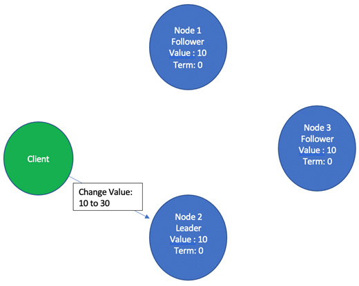
Figure 2.7 – Client requesting the node leader to change the value from 10 to 30

2. When the leader receives this request, it appends this new entry of changing the value from 10 to 30 in its replication log, as illustrated in the following screenshot:

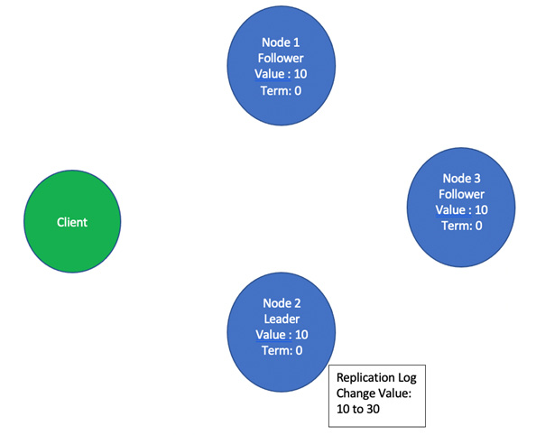
Figure 2.8 – Node 2 appends the entry to change the value from 10 to 30 in its replication log

3. After making an entry in its replication log, it is broadcast to all its followers, as illustrated in the following screenshot:

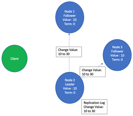
Figure 2.9 – Node 2, the leader, broadcasts this entry of changing the value from 10 to 30 to all its followers

4. All the followers now make an entry in their replication log and acknowledge to the leader that they have done so, as illustrated in the following screenshot:

Figure 2.10 – Followers acknowledge appending the new entry in their own replication logs

5. Once the leader receives an acknowledgment from a majority of the followers, it commits this entry locally and changes the actual node value from 10 to 30, and later broadcasts to all its followers that the entry is committed. This is illustrated in the following screenshot:

Figure 2.11 – Once a majority of the followers acknowledge, the leader commits the changes locally and sends a notification to all its followers about the commit.

6. In the last step, all the followers also commit the entry by changing their node values from 10 to 30, as illustrated in the following screenshot:

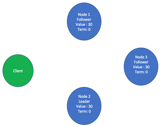
Figure 2.12 – All the followers acknowledge appending the new entry in their own replication logs

This completes the process of log replication for a single change. This process is replayed for all the changes.

If the leader crashes during this negotiation, the replication log can be in an inconsistent state. The new leader fixes this inconsistency by forcing its followers to replicate its own log. Specific details on how this is done are beyond the scope of this book.

Next, we will understand how CockroachDB interacts with the disk.

Interactions with the disk for data storage

The storage layer is responsible for reading from and writing to the disk. Each node in a CockroachDB cluster should have at least one storage attachment. Data is stored as key-value pairs on the disk using a storage engine.

Storage engine

A database management system (DBMS) uses a storage engine to perform CRUD (which stands for create, read, update, and delete) operations on the disk. Usually, the storage engine acts as a black box, so you get more options to choose from based on your own requirements, and also, storage engines evolve independently of the DBMSes that are using them.

Storage engines use a variety of data structures to store data. The popular ones are listed here:

• Hash table
• B+ tree
• Heap
• Log-structured merge-tree (LSM-tree)

Storage engines also work with a wide range of storage types, including the following:

• Solid-state drive (SSD)
• Flash storage
• Hard disk
• Remote storage

CockroachDB primarily supports Pebble as the storage engine, as of version 21.1. Previously, it also supported RocksDB.

Let's look at Pebble.

Pebble

Pebble is primarily a key-value store that provides atomic write batches and snapshots. Starting from version 20.2, CockroachDB uses the Pebble storage engine by default. Pebble was developed to address two concerns, which are outlined here:

• Focusing the storage engine's features to primarily address the requirements of CockroachDB.
• Improving the performance by bringing in certain optimizations that are not part of RocksDB.

Also, since it's developed by Cockroach Labs engineers, it's easy to maintain and control its roadmap. This has also increased the overall productivity as Pebble is written in Golang, just as is CockroachDB itself.

Summary

In this chapter, we learned about all the layers of CockroachDB and how a given request is processed through these layers. We also went through how queries are handled; how a transactional key-value store works; Raft, a distributed consensus algorithm; and a bit about storage engines.

In the next chapter, we will understand ACID and how it's implemented in CockroachDB.