Overview
This chapter aims to show you how to detect faces in an image or a video frame using Haar Cascades, and then track the face when given an input video. Once a face has been detected, you will learn how to use techniques such as GrabCut for performing skin detection. We will also see how cascades can be extended to detect other parts of the face (for instance, the eyes, mouth, and nose). By the end of this chapter, you will be able to create applications for smile detection and Snapchat-like face filters.
Introduction
In the previous chapters, we learned how to use the OpenCV library to carry out basic image and video processing. We also had a look at contour detection in the previous chapter. Now, it's time to take it up a notch and focus on faces – one of the most interesting parts of the human body for computer vision engineers.
Face processing is a hot topic in artificial intelligence because a lot of information can be automatically extracted from faces using computer vision algorithms. The face plays an important role in visual communication because a great deal of nonverbal information, such as identity, intent, and emotion, can be extracted from human faces. This makes it important for you, as a computer vision enthusiast, to understand how to detect and track faces in images and videos and carry out various kinds of filtering operations, for instance, adding sunglasses filters, skin smoothing, and many more, to come up with interesting and significant results.
Whether you want to auto-focus on faces while clicking a selfie or while using portrait mode for pictures, frontal face detection is the foundational technique for building these applications. In this chapter, we will start by understanding the concepts of Haar Cascades and how to use them for frontal face detection. We will also see how we can extend the cascades for detecting features such as eyes, mouths, and noses. Finally, we will learn how to perform skin detection using techniques such as GrabCut and create interesting Snapchat face filters.
Introduction to Haar Cascades
Before we jump into understanding what Haar Cascades are, let's try to understand how we would go about detecting faces. The brute-force method would be to have a window or a block that will slide over the input image, detecting whether there is a face present in that region or not. Detecting whether the block is a face or not can be done by comparing it with some sample face image. Let's see what the issue is with this approach.
The following is a picture of a group of people:

Figure 5.1: Picture of a group of people
Notice the variety of faces in this image. Now, let's look at the following self-explanatory representation of the brute-force method for face detection:

Figure 5.2: Brute-force method for face detection
Here, we can see how difficult it would be if we were to create one standard face that can be used as a reference face to check whether a region in an image has a face or not. For instance, think about the difference in skin tone, facial structure, gender, and other facial features that must be taken into consideration to distinguish faces between people. Another issue with this approach is encountered during the comparison of images. Unlike comparing numerical values, this is a very difficult process. You will have to subtract corresponding pixel values in both images and then see if the values are similar. Let's consider a scenario where both images are the same but have different brightness.
In this case, the pixel values will be very different. Let's consider another scenario where the brightness is the same in the images but the scale (size of the images) is different. A well-known way to deal with this issue is to resize both images to a standard size. Considering all these complexities, you can see that it's very difficult to come up with a general approach to achieve good accuracy by using the basic image processing steps that we learned about in the previous chapters.
To solve this issue, Paul Viola and Michael Jones came up with a machine learning-based approach to object detection in their paper titled Rapid Object Detection Using a Boosted Cascade of Simple Features (https://www.cs.cmu.edu/~efros/courses/LBMV07/Papers/viola-cvpr-01.pdf).
This paper proposed the use of machine learning for extracting relevant features from images. The relevancy here can be described by the role the features play in deciding whether an object is present in the image or not. The authors also came up with a technique called Integral Image for speeding up the computation related to feature extraction in images. Feature extraction was carried out by considering a large set of rectangular regions of different scales, which then move over the image. The trouble with this step, as you can imagine, is the number of features that will be generated by this process. At this step, AdaBoost, a well-known boosting technique, comes into the picture. This technique can reduce the number of features to a great extent and is able to yield only the relevant features out of the huge pool of possible features. Now, we can take this a step further by processing this in a video, which is basically a slideshow of images (termed as frames) within a time period. For instance, based on the quality/purpose of the video, it ranges from 24 frames per second (fps) to 960 fps. Haar Cascades can be used extensively in videos by applying them to each frame.
The basic process for generating such cascades, like any machine learning approach, is data-based. The data here consists of two kinds of images. One set of images doesn't have the object that we want to detect, while the second set of images has the object present in them. The more images you have, and the more variety of images you cover, the better your cascade will be. Let's think about faces here. If you are trying to build a frontal face cascade model, you need to make sure you have a fair share of images for all genders. You will also need to add images with different brightnesses (that is, images taken in the shade or a low-light area versus images taken in bright sunlight). For better accuracy, you would also need to have images showing faces with and without sunglasses, and so on. The aim is to have images that cover a lot of possible varieties.
Using Haar Cascades for Face Detection
Now that we have understood the basic theory behind Haar Cascades, let's understand how we can use Haar Cascades to detect faces in an image with the help of an example. Let's consider the following image as the input image:

Figure 5.3: Input image for the Haar Cascade example
Note
To get the corresponding frontal face detection model, you need to download the haarcascade_frontalface_default.xml trained model (obtained after being trained on a huge number of images with and without faces) from https://packt.live/3dO3RKx.
To import the necessary libraries, you will use the following code:
import cv2
import numpy as np
You have already seen in the previous chapters that the first statement is used for importing a Python wrapper of the OpenCV library. The second statement imports the popular NumPy module, which is used extensively for numerical computations because of its highly optimized implementations.
To load the Haar Cascade, you will use the following code:
haarCascadeFace =
cv2.CascadeClassifier("haarcascade_frontalface_default.xml")
Here, we have used the cv2.CascadeClassifier function, which uses only one input argument – the filename of the XML Haar Cascade model. This returns a CascadeClassifier object.
The CascadeClassifier object has several methods implemented in it, but we will only focus on the detectMultiScale function. Let's have a look at the arguments it takes:
detectedObjects =
cv2.CascadeClassifier.detectMultiScale(image, [scaleFactor,
minNeighbors, flags,
minSize, maxSize])
Here, the only mandatory is the image, which is the grayscale input image in which the faces are to be detected.
The optional arguments are as follows:
scaleFactor decides to what extent the image is going to be resized at every iteration. This helps in detecting faces of different sizes present in the input image. minNeighbors is another argument that decides the minimum number of neighbor's a rectangle should have to be considered for detection. minSize and maxSize specify the minimum and maximum size of the face to be detected. Any face with a size lying outside this range will be ignored.
The output of the function is a list of rectangles (or bounding boxes) that contain the faces present in the image. We can use OpenCV's drawing functions – cv2.rectangle – to draw these rectangles on the image. The following diagram shows the pictorial representation of the steps that need to be followed:

Figure 5.4: Using Haar Cascades for face detection
The following image shows the sample results for different parameter values that have been obtained by performing face detection on Figure 5.3 using the frontal face cascade classifier:

Figure 5.5: The result obtained by using the frontal face cascade classifier
The preceding result is obtained by using the frontal face cascade classifier with scaleFactor = 1.2 and minNeighbors = 9 parameters
Once the parameters have been revised to scaleFactor = 1.2 and minNeighbors = 5, you will notice how the quality of the results obtained degrades. Thus, the results highly depend on the parameter values. The result for the scaleFactor = 1.2 and minNeighbors=5 parameter values would be as follows:

Figure 5.6: The result obtained with the parameters revised to scaleFactor = 1.2 and minNeighbors = 5
Now that we have understood the required functions for performing face detection using Haar Cascades, let's discuss an important concept about bounding boxes before we have a look at an exercise. The bounding box is nothing but a list of four values – x, y, w, and h. x and y denote the coordinates of the top-left corner of the bounding box. w and h denote the width and height of the bounding box, respectively. You can see a diagrammatic representation of this for the cv2.rectangle(img, p1, p2, color) syntax in the following diagram:

Figure 5.7: Plotting a bounding box using OpenCV's rectangle function
Note
Before we go ahead and start working on the exercises and activities in this chapter, please make sure you have completed all the installation steps and set up everything, as instructed in the Preface.
You can download the code files for the exercises and the activities in this chapter using the following link: https://packt.live/2WfR4dZ.
Exercise 5.01: Face Detection Using Haar Cascades
Let's consider a scenario where you must find out the number of students present in a class. One approach is to count the students manually by visiting the class every hour, but let's try and automate this process using computer vision and see whether we can succeed.
In this exercise, we will implement face detection using Haar Cascades. Then, by counting the detected faces, we will see if we can get the number of students present in the class. The observations should focus on the false positives and false negatives discovered. In our scenario, false positive means that a face was not present in the bounding box that the function generated as an output, while false negative means that a face was present, but the cascade failed to detect it.
Since this process does not require a lot of computation, it can be easily carried out at the edge. By edge, we mean that the computation can be carried out at or near the input device, which in our case can be a very simple Raspberry Pi camera that will take a photo every hour, considering that a class in school typically lasts for an hour. Let's consider the following as the input image:

Figure 5.8: Input image
Note
The above image can be found at https://packt.live/2BVgEO5.
Here are the steps we will follow:
- Open a Jupyter notebook, create a new file named Exercise5.01.ipynb, and type out your code in this file.
- Load the required libraries:
import cv2
import numpy as np
- Specify the path of the input image:
Note
Before proceeding, ensure that you can change the path to the image (highlighted) based on where the image is saved in your system.
inputImagePath = "../data/face.jpg"
- Specify the path for the Haar Cascade XML file:
Note
Before proceeding, ensure that you can change the path to the file (highlighted) based on where the file is saved in your system.
haarCascadePath = "../data/haarcascade_frontalface_default.xml"
- Load the image using the cv2.imread function:
inputImage = cv2.imread(inputImagePath)
- Convert the image from BGR mode into grayscale mode using the cv2.cvtColor function:
grayInputImage = cv2.cvtColor(inputImage, cv2.COLOR_BGR2GRAY)
- Load the Haar Cascade:
haarCascade = cv2.CascadeClassifier(haarCascadePath)
- Perform multi-scale face detection using the detectMultiScale function:
detectedFaces = haarCascade.detectMultiScale(grayInputImage, 1.2, 1)
Here, 1.2 is the scaleFactor and 1 is the minNeighbors argument.
- Iterate over all the detected faces and plot a bounding box using the cv2.rectangle function:
for face in detectedFaces:
# Each face is a rectangle representing
# the bounding box around the detected face
x, y, w, h = face
cv2.rectangle(inputImage, (x, y), (x+w, y+h), (0, 0, 255), 3)
Here, detectedFaces is the list of bounding boxes covering the faces present in the image. Thus, the for loop used here iterates over each detected face's bounding box. Then, we used the cv2.rectangle function to plot the bounding box. For this, we passed the image that we want to plot the rectangle on (inputImage), the top left corner of the rectangle (x, y), the bottom right corner of the rectangle (x+w, y+h), the color of the rectangle red = (0, 0, 255), and the line thickness of the rectangle (3) as arguments.
- Use the cv2.imshow function to display the image:
cv2.imshow("Faces Detected", inputImage)
cv2.waitKey(0)
cv2.destroyAllWindows()
Here, the cv2.imshow function will display inputImage in a window with the provided name, "Faces Detected". cv2.waitKey will wait for infinite time (since we have provided 0 as input) until a key is pressed. Finally, the cv2.destroyAllWindows function will close all the windows and the program will exit.
Running the preceding code will result in the following output:

Figure 5.9: Result obtained from face detection using Haar Cascade
You can also save the image using cv2.imwrite so that you can see the image later.
From our observations of the preceding resultant image, we can see that although we were able to detect most of the faces in the image, we still have two false positives and five false negatives.
Note
To access the source code for this specific section, please refer to https://packt.live/3dQwmHw.
Before we proceed to the next section, think about solving the following challenges:
We used a scale factor of 1.2 and a minimum neighbors parameter of 3. Try different values for these parameters and understand their effect on the obtained results. The observations are present in the bounding boxes that the function generated as an output. False negative means that a face was present but the cascade failed to detect it.
Notice that the following image has no false positives. All the bounding boxes that were detected have a face in them. However, the number of faces detected has also reduced significantly here:
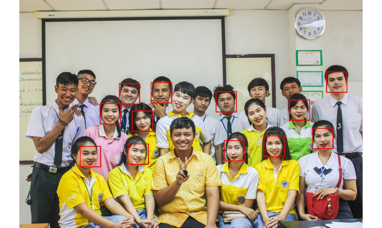
Figure 5.10: Possible resultant image with less detection but no false positives
Compared to the results shown in the preceding image, this following image has detected all the faces in the image successfully, but the number of false positives has increased significantly:

Figure 5.11: Possible resultant image with more detection and more false positives
There is a very common challenge in detection- and tracking-related problems in computer vision called occlusion. Occlusion means that an object is partially or completely covered by another object in the image. Think of it like this – if you are trying to take a selfie but someone comes and stands in front of you, then your image will be occluded by the second person. Now, take two images with you and your friend so that in the first image, both of your faces should be clearly visible, and in the second image, your face should be partially covered by your friend's face. For both images, use the frontal face detection Haar Cascade that we used in this exercise and see if the cascade can detect the occluded face or not. Such tests are always performed for any detection-related models to understand how well suited they are for real-life scenarios.
To understand this better, let's have a look at an example. The following image shows a picture of a soldier and a dog:
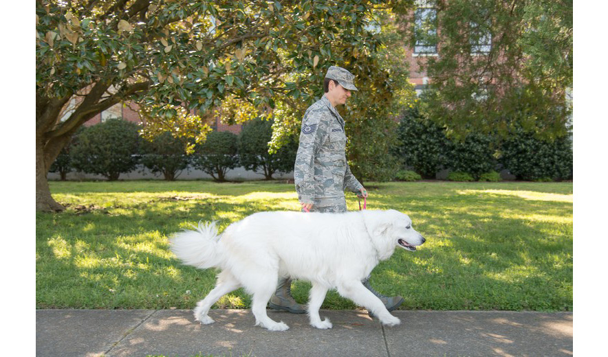
Figure 5.12: Picture of a soldier and a dog
Notice how the dog has partially covered the soldier in this image. Now, we as humans are aware that there is a person behind the dog, but an object detection tool might fail if it has not been trained on similar images.
Detecting Parts of the Face
In the previous section, we discussed face detection and its importance. We also focused on Haar Cascades and how they can be used for object detection problems. One thing that we mentioned but didn't cover in detail was that Haar Cascades can be extended to detect other objects, not just faces.
If you have another look at the methodology for training the cascade model, you will notice that the steps are very general and thus can be extended to any object detection problem. Unfortunately, this requires acquiring a huge number of images, dividing them into two categories based on the presence and absence of the object, and, finally, training the model, which is a computationally expensive process. It is important to note that we cannot use the same haarcascade_frontalface_default.xml file to detect other objects, along with detecting faces at the same time, considering that this model is only trained to detect faces.
This is where OpenCV comes into the picture. OpenCV's GitHub repository has an extensive variety of cascades for detecting objects such as cats, frontal faces, left eyes, right eyes, smiles, and so on. In this section, we will see how we can use those cascades to detect parts of the face, instead of the face itself.
First, let's consider a scenario where detecting parts of the face such as eyes can be important. Imagine that you are building a very basic piece of iris recognition-based biometric security software. The power of this idea can be understood by the fact that the iris of a human being is believed to be much more unique than fingerprints and thus, iris recognition serves as a better means of biometric security. Now, imagine that you have a camera in place at the main gate of your office. Provided that the camera has a high resolution, an eye cascade model will be able to create a bounding box around the eyes present in the video frame. The detected eye regions can then be further processed to carry out iris recognition.
Now, let's try to understand how we can use the various cascade models available online to carry out detection. The process will be very similar to what we have discussed before regarding face detection. Let's take a look:
- To download the relevant model, we will visit OpenCV's GitHub repository at https://packt.live/2VBvtMG.
Note
At the time of writing this chapter, models for detecting eyes, left eyes, right eyes, smiles, and so on were available in this GitHub repository.
- Once the model has been downloaded, the rest of the process will remain the same. We will read the input image.
- As before, the image will have to be converted into grayscale since the cascade model will work only for a grayscale image.
- Next, we will load the cascade classifier model (XML file).
- The only new step will be for multi-scale object detection.
The best part of using Haar Cascades is that you can use the same OpenCV functions every time. This allows us to create a function that will complete all of the preceding steps and return the list of bounding boxes.
Even though the steps that are to be followed remain the same, the importance of parameters increases extensively. After performing Exercise 5.01, Face Detection Using Haar Cascades, and the two challenges, you know that by changing the minimum number of neighbors and the scale factor, the performance of the cascade can be varied. Specifically, in cases where we are trying to detect smaller parts such as eyes, these factors become much more important. As a computer vision engineer, it will be your responsibility to make sure that proper experimentation has been carried out to come up with the parameters that give the best results. In the upcoming exercises, we will see how we can detect eyes in an image, and we will also carry out the required experimentation to get the best set of parameters.
Exercise 5.02: Eye Detection Using Cascades
In this exercise, we will perform eye detection using the haarcascade_eye.xml cascade model.
Note
The image used in this exercise can be found at https://packt.live/3dO3RKx.
Perform the following steps to complete this exercise:
- First, open a Jupyter notebook and create a new file called Exercise5.02.ipynb. Then, type out your code in this file.
- Import the required libraries:
import cv2
import numpy as np
- Load matplotlib, a common Python module for visualization:
Note
For instructions on how to install the matplotlib module, please refer to the Preface.
import matplotlib.pyplot as plt
- Specify the path to the input image and the haarcascade_eye.xml file:
Note
Before proceeding, ensure that you can change the path to the image and file (highlighted) based on where they are saved in the system.
inputImagePath = "../data/eyes.jpeg"
haarCascadePath = "../data/haarcascade_eye.xml"
- Create a custom function to carry out all the steps that we covered in Exercise 5.01, Face Detection Using Haar Cascades:
def detectionUsingCascades(imageFile, cascadeFile):
""" This is a custom function which is responsible
for carrying out object detection using cascade model.
The function takes the cascade filename and the image
filename as the input and returns the list of
bounding boxes around the detected object instances."""
In the next seven steps, we will create this function. This function will also be used in the upcoming exercises and activities.
- Load the image using the cv2.imread function as Step 1 of the detectionUsingCascades custom function:
# Step 1 – Load the image
image = cv2.imread(imageFile)
- Convert the image into grayscale as Step 2 of the detectionUsingCascades custom function:
# Step 2 Convert the image from BGR to Grayscale
gray = cv2.cvtColor(image, cv2.COLOR_BGR2GRAY)
An important point to note here is that you should not convert an image if it is already in grayscale.
- Load the cascade classifier as Step 3 of the detectionUsingCascades custom function:
# Step 3 – Load the cascade
haarCascade = cv2.CascadeClassifier(cascadeFile)
As we saw previously, the cv2.CascadeClassifier function takes in the path to the XML file as input. This path is provided to our custom function, detectionUsingCascades, as an input argument.
- Perform multi-scale detection as Step 4 of the detectionUsingCascades custom function:
# Step 4 – Perform multi-scale detection
detectedObjects = haarCascade.detectMultiScale(gray, 1.2, 2)
Here, it's important to note that detectedObjects is nothing but a list of bounding boxes. Also, note that we have hardcoded the values of the parameters – minNeighbors and scaleFactor. You can either replace these values with better values that you might have obtained from the additional challenges after Exercise 5.01, Face Detection Using Haar Cascades, or you can manually tune these values to obtain the best results. A more finished application would display a set of results for different parameter values and will let the user choose one of the multiple results.
- Draw the bounding boxes using the cv2.rectangle function as Step 5 of the detectionUsingCascades custom function:
# Step 5 – Draw bounding boxes
for bbox in detectedObjects:
# Each bbox is a rectangle representing
# the bounding box around the detected object
x, y, w, h = bbox
cv2.rectangle(image, (x, y), (x+w, y+h),
(0, 0, 255), 3)
- Display the image with bounding boxes drawn over the detected objects as Step 6 of the detectionUsingCascades custom function:
# Step 6 – Display the output
cv2.imshow("Object Detection", image)
cv2.waitKey(0)
cv2.destroyAllWindows()
- Return the bounding boxes as Step 7 of the detectionUsingCascades custom function:
# Step 7 – Return the bounding boxes
return detectedObjects
Note
Depending on your application, the returned bounding boxes can be used for further processing as well.
Now, download the haarcascade_eye.xml file from https://packt.live/3dO3RKx and use the custom function to carry out eye detection on the same input image shown in Figure 5.04:
Note
Before proceeding, ensure that you can change the path to the image and file (highlighted) based on where they are saved in the system.
eyeDetection = detectionUsingCascades("../data/eyes.jpeg",
"../data/haarcascade_eye.xml")
Running the preceding code results in the following output:

Figure 5.13: Result obtained using eye detection
As you can see, though the eyes have been detected, there are many false positives in the preceding result. We will carry out the necessary experimentation to improve the results in Activity 5.01, Eye Detection Using Multiple Cascades.
Note
To access the source code for this specific section, please refer to https://packt.live/2VBrXlj.
You might be wondering why we imported the matplotlib library but never used it. The reason for this is that we want to leave it up to you as a challenge. The finished application that we discussed in Step 9 will use the matplotlib library to create subplots that will have the results for different values of the parameters in a multi-scale detection function. For more details on how to create subplots using matplotlib, you can refer to the documentation at https://matplotlib.org/3.1.1/api/_as_gen/matplotlib.pyplot.subplot.html. Here are a few of the results after varying the minNeighbors parameter:

Figure 5.14: Results after the minNeighbors parameter has been varied
Notice how the results change as the minNeighbors parameter is varied. This experimentation can be carried out by using subplots offered by the matplotlib module.
At this point, let's ponder upon the downsides of cascades. We discussed how cascades are very well suited for operations performed at the edge. Coupled with devices such as Nvidia Jetson, these cascade models can give results with good accuracy and at a very fast speed (that is, for videos, they will have a high FPS).
In such a case, why are industries and researchers moving toward deep learning-based object detection solutions? Deep learning models take a much longer time to train, require more amount of data, and consume a lot of memory for training and sometimes during inference as well. Inference can be thought of as using the model that you got to obtain the results of operations such as object detection. One of the reasons for this is the higher accuracy that is offered by the deep learning models.
Note
As an interesting case study, you can go over this emotion recognition model (https://github.com/oarriaga/face_classification) based on Haar Classifiers, which can give real-time results and does not use deep learning.
Clubbing Cascades for Multiple Object Detection
So far, we've discussed how we can use cascade classifiers to perform object detection. We also discussed the importance of tuning the parameters to obtain better results. We also saw that one cascade model can be used to detect only one object.
If we consider the same iris recognition-based biometric verification case study, we can easily understand that a simple eye detection model is perhaps not the best approach. The reason behind this is that the eye is such a small object to detect that the model will need to check a lot of small regions to confirm if there is an eye present. We saw the same in the results shown in Figure 5.14. A lot of eyes were detected outside the face region. On the other hand, if you consider a face detection model, it will be larger than an eye and thus, we will be able to detect the object (face, in this case) much sooner and with higher accuracy. A better approach in this scenario would be to use a combined model. The steps for the same have been detailed here:
- To detect faces in the image, we will use the face detection model.
- To detect the eye region, we will crop out each face one by one and for each of those cropped faces, we will use the eye detection model.
- To carry out iris recognition, for every detected eye, we can carry out the necessary steps to crop and process the iris region accordingly.
The advantage of using such an approach is that the eye detection model will need to search for an eye in a comparatively smaller region. This was possible only because we were able to use the logic that an eye will be present only in a face. Think of other applications where we can use a similar approach.
In the following activity, we will be resizing the image, which can be done using the cv2.resize function. The function is very easy to use and takes two arguments – the image you want to resize and the new size you want. So, if we have an image called "img" and we want it to resize to 100×100 pixels, we can use newImg = cv2.resize(img, (100,100)).
Activity 5.01: Eye Detection Using Multiple Cascades
We discussed the potential advantage we could get if we used multiple cascades to solve the eye detection problem, instead of directly using the eye cascade. In this activity, you will implement the multiple cascade approach and carry out a comparison between the results obtained using the multiple cascade approach and single cascade approach.
Perform the following steps to complete this activity:
- Create a new Jupyter notebook file called Activity5.01.ipynb.
- Import the necessary Python libraries/modules.
- Download the frontal face cascade and the eye cascade from https://packt.live/3dO3RKx.
- Read the input image and convert it into grayscale.
- Load the frontal face and eye cascade models.
- Use the frontal face cascade model to detect the faces present in the image. Recall that the multi-scale detection will give a list of bounding boxes around the faces as an output.
- Now, iterate over each face that was detected and use the bounding box coordinates to crop the face. Recall that a bounding box is a list of four values – x, y, w, and h. Here, (x, y) is the coordinate of the top-left corner of the bounding box, w is the width, and h is the height of the bounding box.
- For each cropped face, use the eye cascade model to detect the eyes. You can crop the face using simple NumPy array slicing. For example, if a box has the values [x, y, w, h], it can be cropped by using image[y:y+h, x:x+w]:
Figure 5.15: The cropped face obtained using image slicing
- Finally, display the input image with bounding boxes drawn around eyes and faces.
- Now, use the eye cascade model directly to detect eyes in the input image. (This was carried out in Exercise 5.02, Eye Detection Using Cascades.)
- For both cases, perform the necessary experimentation to tune the parameters – scaleFactor and minNeighbors. While you use a manual approach to tune the parameters by running the entire program again and again by changing the parameters, a much better approach would be to iterate over a range of values for both the parameters. As we discussed previously, scaleFactor can be kept as 1.2 as an initial value. Typically, minNeighbors parameter values can be varied from 1 to 9. As an optional exercise, you can try mentioning the number of false positives and false negatives obtained for each experiment that's conducted. Such quantitative figures make your results more convincing.
- Once you have obtained the best possible results using both approaches, try to find any differences in the results obtained using both approaches.
- As an additional exercise to strengthen your understanding of this topic, you can try scaling up the cropped faces (use bilinear interpolation while using the cv2.resize function) to increase the size of the eyes and see if it improves the performance.
The following image shows the expected result of this activity:

Figure 5.16: Result obtained by using multiple cascades
Notice how the results improved significantly compared to the results shown in Figure 5.13.
Note
The solution for this activity can be found on page 497.
One of the problems that deep learning is used to solve is the emotion recognition problem. The basic idea is that, given an image of a face, you have to detect whether the person is happy, sad, angry, or neutral. Think about where this can be used; for example, to build a chatbot that is based on the emotion of the user to interact with them and try improving their mood. Now, of course, it won't be possible for us to solve this problem entirely using cascades because cascades are trained for detection-related problems and not recognition. But we can definitely get a head-start using the cascades. Let's see how. One of the key points that differentiate the various kinds of emotions is a smile. If a person is smiling, we can safely assume that the person is happy. Similarly, the absence of a smile can mean that the person is either angry, sad, or neutral. Notice how we have managed to simplify the recognition problem into a detection problem – specifically, a smile detection problem.
By the end of this activity, you have understood the details of cascades and their implementation for object detection problems. You have also learned how to use multiple cascades instead of just one to improve the performance. You have also carried out various experiments to understand the effect of parameters on the quality of the results obtained. Finally, you will have played around with the scale of the image using OpenCV's resize function to see if the performance improves if the image's size is increased.
Activity 5.02: Smile Detection Using Haar Cascades
In the previous sections, we discussed using cascades and clubbing them to perform eye detection, face detection, and other similar object detection tasks. Now, in this activity, we will consider another object detection problem statement – smile detection.
Luckily for us, there is already a cascade model available in the OpenCV GitHub repository that we can use for our task.
Note
The image and files used in the activity can be found at https://packt.live/3dO3RKx.
We will break down this activity into two parts. The first will be detecting smiles directly using a smile detection cascade, while the second will be clubbing the frontal face cascade and the smile detection cascade.
Perform the following steps to complete this activity:
- Create a new Jupyter notebook file called Activity5.02.ipynb.
- Import the required libraries.
- Next, read the input image and convert it into grayscale (if required).
- Download the haarcascade_smile.xml file from https://packt.live/3dO3RKx.
- Create a variable specifying the path to the smile detection cascade XML file. (You will need this variable to load the cascade.)
- Now, load the cascade using the cv2.CascadeClassifier function. (You will have to provide the path to the XML file as the input argument. This will be the variable you created in the previous step.)
- Next, carry out multi-scale detection, as seen in Exercise 5.02, Eye Detection Using Cascades.
- Create a bounding box around the detected smile and display the final image.
This completes the first part of the activity. Now, use the two cascade classifiers by clubbing them. Perform the following steps to do so:
- Continue in the same file, that is, Activity5.02.ipynb.
- Create a variable specifying the path of the frontal face cascade classifier model.
- Load the classifier by providing the path obtained in the previous step as an argument to the cv2.CascadeClassifier function.
- Carry out multi-scale detection to detect the faces in the image.
- Iterate over each face and crop it. Use the steps provided in Activity 5.01, Eye Detection Using Multiple Cascades, as a reference.
- For each face, use the smile detection cascade classifier to detect a smile.
- Create a bounding box over the detected smile.
This way, you should have a bounding box over each face and for each face, a bounding box over the detected smile, as seen here:

Figure 5.17: Result obtained by using the frontal face and smile cascade classifiers
Note
The solution for this activity can be found on page 500.
This completes the entire activity. What do you think? Can you use this method to recognize whether a person is happy or not? The biggest drawback of the technique we discussed in this activity is that it assumes that a smile is enough to tell us whether a person is happy or not. There are other parts of the face such as facial muscles that come into the picture in regard to recognizing the emotion of a face. That's why deep learning models surpass simple machine learning models in these cases as they can take into account a large number of features to predict the output.
We can also replace the input image with a video stream from a webcam or a recorded video file using OpenCV functions such as cv2.VideoCapture(0) and cv2.VideoCapture('recorded_video_file_name'), respectively. Once you take inputs from the video stream, you will notice the performance of the technique as you make different faces. We will complete an interesting activity using a webcam at the end of this chapter.
In later chapters, we will discuss facial recognition using deep learning techniques where we will revisit this problem statement of emotion recognition and compare the performance of the cascade-based technique and deep learning-based technique.
In the next section, we will discuss a very important technique called GrabCut and how we can use it for skin detection problems.
GrabCut Technique
Before we go into the details of this amazing technique, we need to understand the term Image Segmentation, which will form the very basis of GrabCut. In layman's terms, an image segmentation task comprises dividing the pixels into different categories based on the class they belong to. Here, the classes we are looking for are just the background and foreground. This means that we want to segment the image by deciding what region of the image is part of the background and what region of the image is part of the foreground.
Note
In deep learning, image segmentation is a very big topic and is comprised of segmenting an image based on its classes, sometimes based on semantics, and so on. For now, we can consider GrabCut a simple background removal technique, though technically it can also be considered as an image segmentation technique with only two primary classes in mind – background and foreground. It's also important to note here that GrabCut uses not two, but four labels that we will discuss later in this section. But the basic idea will stay the same – remove the background from the image.
For example, consider the following image:

Figure 5.18: Person in a garden doing some exercise
If we focus on the foreground and background, we can say that the background is the garden or park in which the person is exercising, and the foreground consists of the person in the picture. Taking this into account, if we go ahead and perform image segmentation, we will end up with the following image:

Figure 5.19: Result after performing image segmentation
Notice how only the foreground is present in the image. The entire background has been removed and replaced with white pixels (or white background).
Hopefully, by now, some ideas have started popping up in your mind regarding where you can use this technique. For Adobe Photoshop users, a similar technique is used quite extensively in photo editing. The idea of green screen used in movies is also based on a similar concept.
Now, let's go into the details of the GrabCut technique. GrabCut was a technique for interactive foreground extraction (a fancy phrase meaning that a user can interactively extract foreground) proposed by Carsten Rother, Vladimir Kolmogorov, and Andrew Blake in their paper "GrabCut" – Interactive Foreground Extraction using Iterated Graph Cuts (http://pages.cs.wisc.edu/~dyer/cs534-fall11/papers/grabcut-rother.pdf). The algorithm used color, contrast, and user input to come up with excellent results.
The power of the algorithm can be understood by the number of applications built on top of it. While it might seem a manual procedure at first glance, the fact is that the manual part comes into the picture only to provide finishing to the results or to improve them further. Also, refer to the paper Automatic Skin Lesion Segmentation Using GrabCut in HSV Color Space by Fakrul Islam Tushar (https://arxiv.org/ftp/arxiv/papers/1810/1810.00871.pdf). This work is a very good example that shows the true power of GrabCut. The smart use of the HSV color space (refer to Chapter 2, Common Operations When Working with Images, for details regarding color spaces) instead of the usual BGR color space along with GrabCut's iterative procedure managed to segment (or separate) the skin lesion. As the paper mentions, this is the first step toward a digital and automatic diagnosis of skin cancer.
In the coming sections, we will use GrabCut to segment a person from an image for skin detection, which will then be used in the final activity of this chapter to create various face-based filters.
Note
Saving an image is an important step in computer vision and can be carried out using the cv2.imwrite function. The function takes two arguments – the name of the file and the image we want to save.
To carry out GrabCut, we will use the cv2.grabCut() function. The function syntax looks as follows:
outputmask, bgModel, fgModel = cv2.grabCut(image, mask,
rect, bgModel, fgModel, iterCount, mode)
Let's understand each of these arguments:
image is the input image we want to carry out GrabCut on. iterCount is the number of iterations of GrabCut you want to run. bgModel and fgModel are just two temporary arrays used by the algorithm and are simply two arrays of size (1, 65).
There are four possible modes, but we will only focus on the two important ones, that is, mask and rect. You can read about the rest of them at https://docs.opencv.org/3.4/d7/d1b/group__imgproc__misc.html#gaf8b5832ba85e59fc7a98a2afd034e558. Let's take a look at them:
cv2.GC_INIT_WITH_RECT mode means that you are initializing your GrabCut algorithm using a rectangular mask specified by the rect argument. cv2.GC_INIT_WITH_MASK mode means that you are initializing your GrabCut algorithm with a general mask (a binary image, basically) specified by the mask input argument. mask has the same shape as the image provided as input.
The function returns three values. Out of the three values, the only important one for us is outputmask, which is a grayscale image of the same size as the image provided as input but has only the following four possible pixel values:
Pixel value 0 or cv2.GC_BGD means that the pixel surely belongs to the background. Pixel value 1 or cv2.GC_FGD means that the pixel surely belongs to the foreground. Pixel value 2 or cv2.GC_PR_BGD means that the pixel probably belongs to the background. Pixel value 3 or cv2.GC_PR_FGD means that the pixel probably belongs to the foreground.
One more important function that we will be using extensively is OpenCV's cv2.selectROI function to select a rectangular region of interest when we are using the cv2.GC_INIT_WITH_RECT mode. The usage of the function is very simple. You can directly use your mouse to select the top-left corner and then drag your cursor to select the rectangle. Once done, you can press the Spacebar key to get the ROI.
Similarly, we use a Sketcher class, which has been provided in the upcoming exercises, to modify the mask interactively. We can download the class directly from OpenCV samples: https://github.com/opencv/opencv/blob/master/samples/python/common.py. You don't need to understand the details of this class, except that it lets us sketch an image using our mouse. The Sketcher class can be called as follows:
sketch = Sketcher('image', [img, mask],
lambda : ((255,0,0), 255))
Here, 'image' is the name of the display window that will pop up, and img and mask are two images that will be displayed – one where you will be sketching (img) and the other where the result is displayed automatically (mask). (255,0,0) means that when we sketch on img, we will be drawing in blue.
The 255 value means that whatever we draw on img will be displayed on mask in white. You can guess here that img is a BGR image, whereas mask is a grayscale image.
Once you have obtained the output mask, you can multiply it with your input image, which will give you only the foreground and remove the background from the image.
We will go into details of this topic with the help of a couple of exercises and then finally take up skin detection as an activity.
Exercise 5.03: Human Body Segmentation Using GrabCut with Rectangular Mask
In this exercise, we will carry out foreground extraction to segment a person from the input image. We will use the cv2.GC_INIT_WITH_MASK mode in this problem with Figure 5.20 as the input image.
Note
The image can be found at https://packt.live/2VzJ1bv.
Perform the following steps to complete this exercise:
- Open your Jupyter notebook, create a new file called Exercise5.03.ipynb, and write your code in this file.
- Import the required libraries:
import cv2
import numpy as np
- Read the input image:
Note
Before proceeding, ensure that you can change the path to the image (highlighted) based on where the image is saved in your system.
# Read image
img = cv2.imread("../data/person.jpg")
- Create a copy of the image:
imgCopy = img.copy()
- Create a mask of the same size (width and height) as the original image and initialize mask with zeros using NumPy's np.zeros function. Also, specify the data type as an unsigned 8-bit integer, as shown in the following code:
# Create a mask
mask = np.zeros(img.shape[:2], np.uint8)
- Create two temporary arrays:
# Temporary arrays
bgdModel = np.zeros((1,65),np.float64)
fgdModel = np.zeros((1,65),np.float64)
- Use OpenCV's cv2.selectROI function to select the region of interest:
# Select ROI
rect = cv2.selectROI(img)
- Draw the rectangle over the ROI and save the image:
# Draw rectangle
x,y,w,h = rect
cv2.rectangle(imgCopy, (x, y), (x+w, y+h),
(0, 0, 255), 3)
cv2.imwrite("roi.png",imgCopy)
Running the preceding code will result in the following output:

Figure 5.20: Region of interest selected using the cv2.SelectROI function
- Next, we will perform GrabCut using cv2.grabCut:
# Perform grabcut
cv2.grabCut(img,mask,rect,bgdModel,fgdModel,5,cv2.GC_INIT_WITH_RECT)
- Include all the confirmed and probable background pixels in the background by setting these pixels as 0:
mask2 = np.where((mask==2)|(mask==0),0,1).astype('uint8')
- Display both mask and mask2 using the following code:
mask2 = np.where((mask==2)|(mask==0),0,1).astype('uint8')
cv2.imshow("Mask",mask*80)
cv2.imshow("Mask2",mask2*255)
cv2.imwrite("mask.png",mask*80)
cv2.imwrite("mask2.png",mask2*255)
cv2.waitKey(0)
The following shows the mask that was obtained after using the GrabCut operation:

Figure 5.21: Mask obtained after using the GrabCut operation
The brighter regions correspond to the confirmed foreground pixels, while the grey regions correspond to the probably background pixels. Black pixels are guaranteed to belong to the background.
The following image shows the mask that was obtained after combining the confirmed background pixels and probable background pixels:

Figure 5.22: Mask obtained after combining the confirmed background pixels and probable background pixels
The white region corresponds to the foreground. Unfortunately, the mask does not provide us with much information.
- Multiply the mask with the image to obtain only the foreground using the following code:
img = img*mask2[:,:,np.newaxis]
We are introducing a new axis to simply match the shapes.
- Display and save the final image using the following code:
cv2.imwrite("grabcut-result.png",img)
cv2.imshow("Image",img)
cv2.waitKey(0)
cv2.destroyAllWindows()
Running the preceding code displays the following output:

Figure 5.23: Foreground detected using GrabCut
Notice that though the result is of good quality, the shoes of the person are detected as the background.
Note
To access the source code for this specific section, please refer to https://packt.live/31AjOBE.
In Figure 5.23, we noticed how the GrabCut technique provided good results, but it still needed a finer touch. At this stage, there are two ways to improve the result:
- You can try changing the iterCount parameter in the cv2.grabCut function to see if the quality of the result improves:

Figure 5.24: Result obtained after running GrabCut for only one iteration
Notice that the shoes are still in the background and there is some additional grass that has been detected as part of the foreground.
- You can try selecting different ROIs to see if there is any difference in the result obtained.
But as you will see after experimenting, using these suggestions, there is no significant improvement in the result obtained using GrabCut. One option that can be used at this step is to modify the mask manually and provide it again as input to the GrabCut process for better results. We will see how to do that in the next exercise.
Exercise 5.04: Human Body Segmentation Using Mask and ROI
In the previous exercise, we saw how GrabCut was very easy to use but that the results needed some improvement. In this exercise, we will start by using a rectangular ROI mask to perform segmentation with GrabCut and then add some finishing touches to the mask to obtain a better result. We will be using Figure 5.3 as the input image.
Note
The image can be found at https://packt.live/2BT1dFZ.
Perform the following steps to complete this exercise:
- Open your Jupyter notebook, create a new file called Exercise5.04.ipynb, and start writing your code in this file.
- Import the required libraries:
import cv2
import numpy as np
- Read the input image:
Note
Before proceeding, ensure that you can change the path to the image (highlighted) based on where the image is saved in your system.
# Read image
img = cv2.imread("../data/grabcut.jpg")
- Create a copy of the input image:
imgCopy = img.copy()
- Create a mask of the same size as the input image, initialize it with zeros, and use unsigned 8-bit integers, as shown in the following code:
# Create a mask
mask = np.zeros(img.shape[:2], np.uint8)
- Create two temporary arrays:
# Temporary arrays
bgdModel = np.zeros((1,65),np.float64)
fgdModel = np.zeros((1,65),np.float64)
- Select a rectangular ROI to perform a crude GrabCut operation:
# Select ROI
rect = cv2.selectROI(img)
Running the preceding code will display the following output:

Figure 5.25: The GUI for selecting ROI using the cv2.selectROI function
- Draw the rectangle on the copy of the input image and save it:
# Draw rectangle
x,y,w,h = rect
cv2.rectangle(imgCopy, (x, y), (x+w, y+h),
(0, 0, 255), 3)
cv2.imwrite("roi.png",imgCopy)
The following image will be saved as roi.png:

Figure 5.26: Final rectangular ROI selected for GrabCut
- Next, perform the GrabCut operation, as we saw in the previous exercise:
# Perform grabcut
cv2.grabCut(img,mask,rect,bgdModel,fgdModel,5,cv2.GC_INIT_WITH_RECT)
- Use both confirmed background and probable background pixels in the output mask as background pixels:
mask2 = np.where((mask==2)|(mask==0),0,1).astype('uint8')
- Display and save both masks:
cv2.imshow("Mask",mask*80)
cv2.imshow("Mask2",mask2*255)
cv2.imwrite("mask.png",mask*80)
cv2.imwrite("mask2.png",mask2*255)
cv2.waitKey(0)
cv2.destroyAllWindows()
Note that we are multiplying mask by 80 since the pixel values in mask range only from 0 to 3 (inclusive) and thus won't be visible directly. Similarly, we are multiplying mask2 by 255.
The following image shows the mask obtained after performing GrabCut:

Figure 5.27: Mask obtained after performing the GrabCut operation
The brighter regions correspond to the confirmed foreground pixels, while the grey regions correspond to the probable background pixels. Black pixels are guaranteed to belong to the background.
The following image shows the mask that was obtained after clubbing the confirmed background and probable background pixels into the background pixels category:
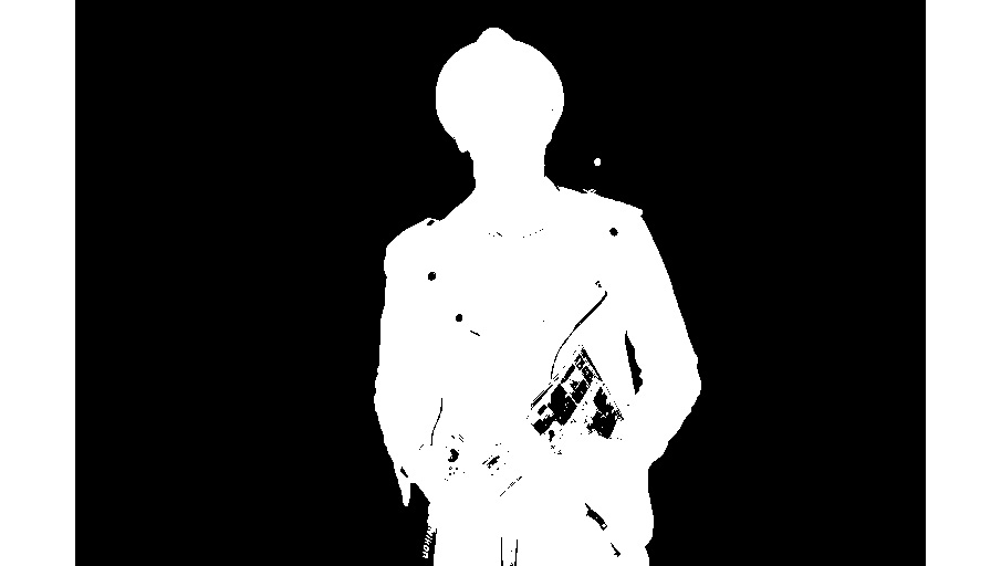
Figure 5.28: Mask is obtained after clubbing the confirmed background
The preceding mask is obtained after clubbing the confirmed background and probable background pixels into the background pixels category.
Notice the white spot outside of the human body region and several black regions inside the foreground region. These patches will now need to be fixed.
- Multiply the image with mask2 to obtain the foreground region:
img = img*mask2[:,:,np.newaxis]
- At this stage, create a copy of the mask and the image:
img_mask = img.copy()
mask2 = mask2*255
mask_copy = mask2.copy()
We are multiplying mask2 by 255 because of the same reason mentioned in Step 11.
- Use the Sketcher class provided by OpenCV for mouse handling. Using this class, modify the mask (that is, the foreground and background) with the help of your cursor:
# OpenCV Utility Class for Mouse Handling
class Sketcher:
def __init__(self, windowname, dests, colors_func):
self.prev_pt = None
self.windowname = windowname
self.dests = dests
self.colors_func = colors_func
self.dirty = False
self.show()
cv2.setMouseCallback(self.windowname, self.on_mouse)
We will be able to see the change in the result dynamically using this process. The preceding function, that is, __init__, initializes the Sketcher class object.
- Use the show function to display the windows:
def show(self):
cv2.imshow(self.windowname, self.dests[0])
cv2.imshow(self.windowname + ": mask", self.dests[1])
- Use the on_mouse function for mouse handling:
# onMouse function for Mouse Handling
def on_mouse(self, event, x, y, flags, param):
pt = (x, y)
if event == cv2.EVENT_LBUTTONDOWN:
self.prev_pt = pt
elif event == cv2.EVENT_LBUTTONUP:
self.prev_pt = None
if self.prev_pt and flags & cv2.EVENT_FLAG_LBUTTON:
for dst, color in zip(self.dests, self.colors_func()):
cv2.line(dst, self.prev_pt, pt, color, 5)
self.dirty = True
self.prev_pt = pt
self.show()
- Create a sketch using the Sketcher class, as shown here:
# Create sketch using OpenCV Utility Class: Sketcher
sketch = Sketcher('image', [img_mask, mask2], lambda : ((255,0,0), 255))
The parameters for the lambda function mean that any blue pixel (255,0,0) drawn in the image will be displayed as a white pixel (255) in the mask.
- Next, create an infinite while loop since we want to modify the mask, and thus the results, for as long as we want. Use the cv2.waitKey() function to keep a record of the key that's been pressed:
while True:
ch = cv2.waitKey()
# Quit
if ch == 27:
print("exiting...")
cv2.imwrite("img_mask_grabcut.png",img_mask)
cv2.imwrite("mask_grabcut.png",mask2)
break
# Reset
elif ch == ord('r'):
print("resetting...")
img_mask = img.copy()
mask2 = mask_copy.copy()
sketch = Sketcher('image', [img_mask, mask2],
lambda : ((255,0,0), 255))
sketch.show()
If the Esc key is pressed, we will break out of the while loop after saving both the mask and the image and if the R key is pressed, we will reset the mask and the image.
- Use blue (255,0,0) to select the foreground and red (0,0,255) to select the background:
# Change to background
elif ch == ord('b'):
print("drawing background...")
sketch = Sketcher('image', [img_mask, mask2],
lambda : ((0,0,255), 0))
sketch.show()
# Change to foreground
elif ch == ord('f'):
print("drawing foreground...")
sketch = Sketcher('image', [img_mask, mask2],
lambda : ((255,0,0), 255))
sketch.show()
A background pixel in mask will be marked as black (0). By pressing F and B, you can switch between the foreground and background selections, respectively.
The result that's obtained by using the preceding code can be seen here:
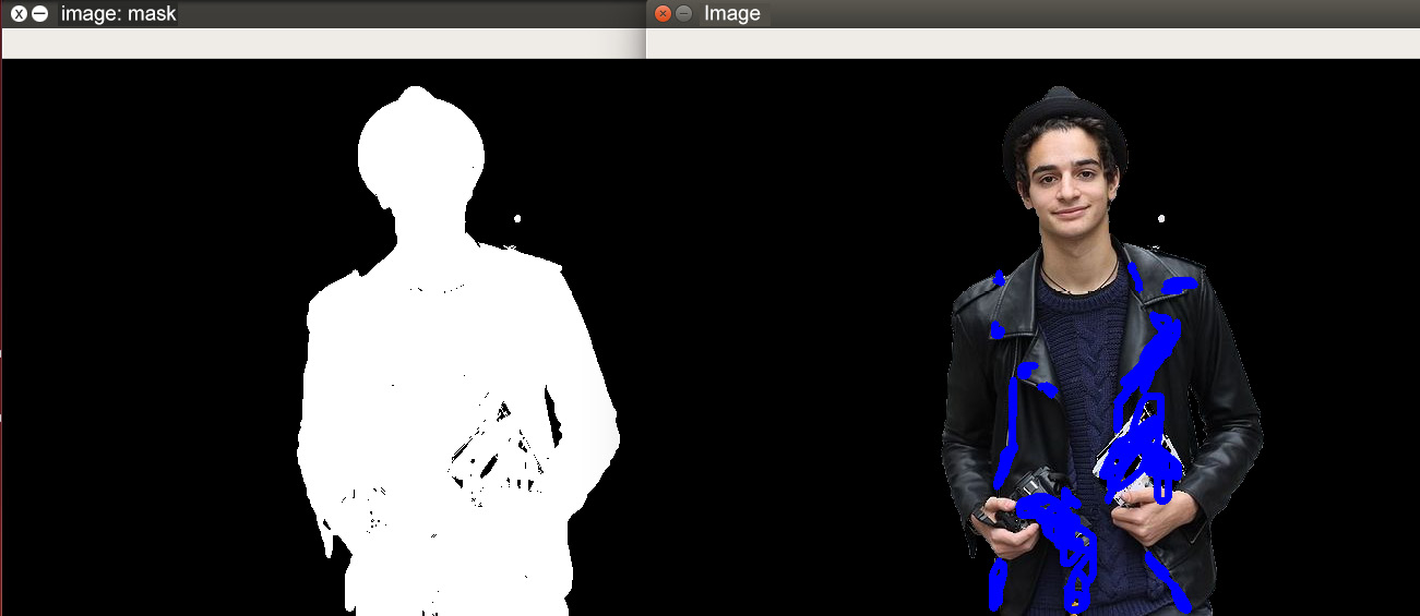
Figure 5.29: The foreground region correction marked in blue
The foreground region correction is marked in blue as this covers the black patches that were present in the mask in the foreground region shown in Figure 5.27. The regions marked in blue will now become a part of the foreground in the mask, which means they will now become white in the mask, as can be seen in the preceding image on the left.
The following image shows the background correction marked in red:
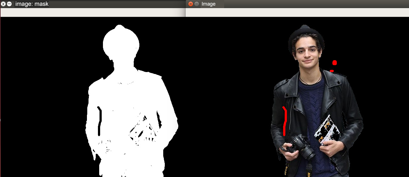
Figure 5.30: The background correction marked in red
Similar to the foreground correction, the background correction is marked in red. The marked region comprises the areas that truly belonged to the background but was labeled as foreground by GrabCut. These regions will be labeled as black in the mask. The same can be seen in the image on the left-hand side.
- Carry out the GrabCut operation using the revised mask, in case any other key is pressed:
else:
print("performing grabcut...")
mask2 = mask2//255
cv2.grabCut(img,mask2,None,
bgdModel,fgdModel,5,cv2.GC_INIT_WITH_MASK)
mask2 = np.where((mask2==2)|(mask2==0),0,1)
.astype('uint8')
img_mask = img*mask2[:,:,np.newaxis]
mask2 = mask2*255
print("switching bank to foreground...")
sketch = Sketcher('image', [img_mask, mask2],
lambda : ((255,0,0), 255))
sketch.show()
Note that we are now using the cv2.GC_INIT_WITH_MASK mode since we are providing the mask instead of the ROI rectangle.
- Close all the open windows and exit, once you are out of the while loop:
cv2.destroyAllWindows()
The following image shows the final mask that was obtained after foreground and background correction:

Figure 5.31: The final mask that was obtained after foreground and background correction
- Compare the following final corrected image with the mask displayed in Figure 5.27 to understand the corrections made:

Figure 5.32: The final image obtained after the corrections
This was a long exercise. Let's quickly summarize what we did in this exercise. First, we performed a crude GrabCut using a rectangular ROI. The mask was then corrected with the help of the Sketcher class. The corrections were broken down into two parts – foreground correction and background correction. The mask that was obtained was then used again by GrabCut to obtain the final foreground image.
Note
To access the source code for this specific section, please refer to https://packt.live/2NMv6dS.
Activity 5.03: Skin Segmentation Using GrabCut
You must have watched those James Bond-type movies where a villain would put on a mask of the hero and commit a crime. Well, so far, we have learned how to detect faces and noses, but how do we crop out skin regions? In this activity, you will implement skin segmentation using the GrabCut technique. We will use the same code that we developed in the previous exercise and modify it slightly to create a frontal face cascade classifier to detect faces. You can also use the previous exercise as a reference to modify the mask using the mouse.
Let's learn how to carry out this activity:
- Open your Jupyter notebook and create a new file called Activity5.03.ipynb.
- Import the OpenCV and NumPy modules.
- Add the code for the Sketcher class first as we will be using it in this activity to revise the mask obtained by GrabCut.
- Read the input image, that is, "grabcut.jpg", using the cv2.imread function. This is the same image that we used in the previous exercise.
Note
The image can be found at https://packt.live/2BT1dFZ.
- Convert the BGR image into grayscale mode using the cv2.cvtColor function.
- Now, load the Haar Cascade for frontal face detection using the cv2.CascadeClassifier function.
- Use the cascade classifier to detect a face in the image using the detectMultiScale function. Select the parameter values so that only the correct face is detected.
- Use the bounding box obtained in the preceding step to crop the face from the image.
- Now, resize the image and increase its dimensions to 3x. For this, you can use the cv2.resize function. We will now be working on this resized image.
- Use the cv2.grabCut function to obtain the mask. The sample result can be seen here:

Figure 5.33: The mask obtained using the GrabCut function
- Now, club the confirmed background and probable background pixels into confirmed background pixels. The following image shows the sample result:

Figure 5.34: The mask obtained after clubbing the background and probable background pixels
- Next, multiply the new mask with the image to obtain the foreground.
- Now, use the steps described in the previous exercise to obtain a revised mask and finally the skin region:

Figure 5.35: Mask obtained after foreground and background correction
The segmented skin region will look as follows:

Figure 5.36: Segmented skin region
Note
The solution for this activity can be found on page 503.
To summarize, in this activity, we used frontal face cascade classifiers along with the GrabCut technique to perform skin segmentation.
Now, it's time to move on to the final activity of this chapter. In this activity, we will build an emoji filter, similar to Snapchat filters, using the techniques we studied in this chapter.
Activity 5.04: Emoji Filter
Whether it is Instagram, Facebook, or Snapchat, filters have always been in demand. In this activity, we will build an emoji filter using the techniques we have discussed in this chapter. With the help of the previously discussed VideoCapture function, use the input from your webcam.
Here are the steps you need to follow:
- Open your Jupyter notebook and create a new file called Activity5.04.ipynb.
- Import the OpenCV and NumPy modules.
- Write the function responsible for applying the emoji filter. To start, copy the detectionUsingCascades function that we wrote in Exercise 5.02, Eye Detection Using Cascades. Modify this function slightly for this case study activity.
- Change the function name to emojiFilter and add a new argument to it called emojiFile, which is the path to the emoji image file.
- Inside the emojiFilter function, in Step 1 (similar to how we did for the custom function earlier), add the code to read the emoji image using the cv2.imread function. Make sure you pass –1 as the second argument since we also want to read the alpha channel in the image, which is responsible for transparency in images. We will also be providing the image directly as the first argument instead of the image file name, so remove the cv2.imread function call for reading the image.
- There is no modification required in Steps 2 and 3.
- Add an if-else condition to check if any object is even detected using the Haar Cascade in Step 4. If no object is detected, return None.
- In Step 5, resize our emoji so that it matches the size of the detected face. The size of the detected face is nothing but (w, h). For resizing, use the cv2.resize function, as we did previously.
- Once the emoji has been resized, we will need to replace the face with the emoji. This is where the alpha channel comes into the picture. Our image has 100% transparency for the background and 0% transparency for the actual emoji region. The 100% transparency region will have a value of 0 (black region) in the alpha channel. You can use the following code as a reference:
(image[y:y+h, x:x+w])[np.where(emoji_resized[:,:,3]!=0)] =
(emoji_resized[:,:,:3])[np.where(emoji_resized[:,:,3]!=0)]
The output is as follows:

Figure 5.37: An emoji that we are going to use in our emoji filter
Note
The image can be found at https://packt.live/3evTz1L.
The alpha channel of the emoji will look as follows:

Figure 5.38: Alpha channel of the emoji we are using
- We will exploit the fact mentioned in Step 9 to overwrite only regions of the face corresponding to the non-transparent regions of the face with those non-transparent pixels.
- Also, revise the function to return the final image instead of detected objects.
- Now, since we are going to take input from a webcam, we will have to write some code for starting the webcam, capturing the frames, and then displaying the output.
- Create a VideoCapture object using cv2.VideoCapture. Pass the only required argument as 0 since we want to take input from the webcam. If you wanted to provide input from a video file, you could have provided the filename. Name the VideoCapture object cap.
- Now, create a while loop and in the loop, use cap.read() to capture a frame from the webcam. This returns two values – a return value signifying whether the frame capture was successful or not, and the captured frame.
- If the return value from cap.read() was True, meaning that the frame was read successfully, pass it to the emojiFilter function and display the output using the cv2.imshow and cv2.waitKey functions. Provide a non-zero value as an argument to the cv2.waitKey function, since we don't want to wait infinitely long for the next frame to be displayed. Use a value of 10 or 20:

Figure 5.39: Sample output of the emoji filter on a single frame
Note
The output shown in the preceding image has been generated using a pre-recorded video and not the webcam. We would recommend that you use your webcam to generate interesting results and only treat the preceding image as a reference.
Similar outputs will be generated for each frame of the video.
Note
The solution for this activity can be found on page 509.
That's it. You have prepared your own emoji filter. Of course, it's not a very good-looking filter, but it's a start. You can now make this much more interesting by switching between different emojis randomly or based on the presence of a smile. Switching between happy and sad emojis based on smile detection can help you build your own emotion detector emoji filter. Similarly, you can add other transparent images to the frames to give some nice makeup to your emoji. Once you have gathered and practiced the basic idea, the sky is the limit for you.
Summary
In this chapter, we started off by seeing why the face is considered an important source that's used to identify different emotions, features, and so on. We also discussed why we cannot have a simple face-matching algorithm because of the large variety of faces available to us. We then approached the topic of Haar Cascades and built several applications using one or multiple cascade classifiers. We also talked in detail about the importance of experimentation when it comes to obtaining a set of arguments that will give us the best results using cascade classifiers. After that, we discussed the GrabCut technique and built a human body segmentation application using a rectangular ROI mask. After that, we modified the code to allow the user to correct the mask to obtain better results. We then covered how to carry out skin segmentation using GrabCut and finally ended the chapter with the emoji filter, which can be run on an input video taken from a webcam or a video file.
From the next chapter onward, we will start looking at the advanced topics of computer vision. The first topic we will be covering is object tracking, which will allow the user to track the motion of a selected object in a video. We will also discuss the various trackers available in OpenCV and discuss the differences between their performance.