Overview
This chapter will familiarize you with the concept of contours. You will learn how to detect nested contours and access specific contours with a given shape or moment distribution. You will gain the ability to play with contours. This ability will come in handy during object detection tasks, especially when you are searching and selecting your object of interest. You will also learn how to access contours according to their hierarchy. Moreover, you'll learn how to fetch contours of a particular shape from an image with multiple contours. By the end of this chapter, you will be able to detect and handle contours of different shapes and sizes.
Introduction
In the previous chapter, we learned about histogram equalization, which was used to enhance an image by bringing out the hidden details in a dark image. In this chapter, we will learn how to fetch objects of interest from an image. We will start with a gentle introduction to contours and then move ahead to see some interesting ways in which you can apply this concept. A contour is the boundary of an object – it is a closed shape along the portion of an image that has the same color or intensity. Speaking in terms of OpenCV, a contour is the boundary of a group of white pixels on a black background. Yes, in OpenCV, contours can be extracted only from binary images.
In practical terms, contours can help you to count the number of objects in an image. You can also use contours to identify your object(s) of interest in a given image, for example, to detect a basketball net in an image (Exercise 4.05, Detecting a Basketball Net in an Image). Furthermore, you will find that contour detection can be used to identify objects with a particular height or width ratio (you will find a use case for this in Exercise 4.06, Detecting Fruits in an Image).
This chapter provides a walkthrough of how contours can be detected, plotted, and counted. You will see what the difference is between contours and edges. You will learn about contour hierarchy, how to access different contours, and how to find contours of a given reference shape in an image with multiple contours. It will be an interesting journey and will equip you with a solid skill set before you venture out on your image processing adventures.
Contours – Basic Detection and Plotting
A contour can only be detected in a binary image using OpenCV. To detect contours in colored (BGR) or grayscale images, you will first need to convert them to binary.
Note
In OpenCV, a colored image has its channels in the order of BGR (blue, green, and red) instead of RGB.
To find the contours in a colored image, first, you will need to convert it to grayscale. After that, you will segment it to convert it to binary. This segmentation can be done either with thresholding based on a fixed grayscale value of your choice or by using Otsu's method (or any other method that suits your data). Following is a flowchart of contour detection:

Figure 4.1: Flowchart of contour detection
The command to detect contours in an image is as follows:
contours, hierarchy = cv2.findContours(source_image,
retrieval_mode, approx_method)
There are two outputs of this function:
- contours is a list containing all detected contours in the source image.
- hierarchy is a variable that tells you the relationship between contours. For example, is a contour enclosed within another? If yes, then is that larger contour located within a still larger contour?
In this section, we will just explore the contours output variable. We will explore the hierarchy variable in detail in the Hierarchy section.
Here is a brief explanation of the inputs of this function:
- source_image is your input binary image. To detect contours, the background of this binary image must be black. Contours are extracted from white blobs.
- retrieval_mode is a flag that instructs the cv2.findContours function on how to fetch all contours. (Should all contours be fetched independently? If a contour lies inside another larger contour, should that information be returned? If many contours lie inside a larger contour, should the internal contours be returned, or will just the outer contour suffice?)
If you only want to fetch all the extreme outer contours, then you should keep it to be cv2.RETR_EXTERNAL. This will ignore all those contours that lie inside other contours.
If you simply want to retrieve all contours independently and do not care which lies inside which one, then cv2.RETR_LIST would be your go-to choice. This does not create parent-child relationships and so all contours are at the same hierarchical level.
If you are interested in finding the outer and inner boundaries of objects (two levels only: the border of the outer shape and the boundary of the inner hole), then you would go for cv2.RETR_CCOMP.
If you want to make a detailed family tree covering all generations (parent, child, grandchild, and great-grandchild), then you need to set this input as cv2.RETR_TREE.
- approx_method is a flag that tells this function how to store the boundary points of a detected contour. (Should each coordinate point be saved? If so, keep this flag's value as cv2.CHAIN_APPROX_NONE. Or should only those points be saved that are strictly needed to draw the contour? In that case, set the flag to cv2.CHAIN_APPROX_SIMPLE. This will save you a lot of memory.) If you want to dig into this further, do check out https://opencv-python-tutroals.readthedocs.io/en/latest/py_tutorials/py_imgproc/py_contours/py_contours_begin/py_contours_begin.html.
Suppose you have an image of silhouettes (as shown in the following screenshot) and you need to detect contours on it:

Figure 4.2: Sample binary image
We can store the preceding image in an img variable. Then to detect contours, we can apply the cv2.findContours command. For the sake of this introductory example, we will use external contour detection and the CHAIN_APPROX_NONE method:
contours, hierarchy = cv2.findContours(img, cv2.RETR_EXTERNAL,
cv2.CHAIN_APPROX_NONE)
To plot the detected contours on a BGR image, the command is as follows:
marked_img = cv2.drawContours(img, contours, contourIdx, color,
thickness, lineType = cv.LINE_8,
hierarchy = new cv.Mat(),
maxLevel = INT_MAX,
offset = new cv.Point(0, 0)))
The output of this function is the image, img, with the contours drawn on it.
Here is a brief explanation of the inputs of this function:
- img is the BGR version of the image on which you want the contours to be marked. It should be BGR because you will need to draw the contours with some color other than black or white and the color will have three values in its BGR code. So, you will need three channels in the image.
- contours is the Python list of detected contours.
- contourIdx is the contour you want to draw from the list of contours. If you want to draw all of them, then its input value will be -1.
- color is the BGR color code of the color you want to use for plotting. For example, for red it will be (0, 0, 255). To see the RGB color codes for some commonly used colors, visit https://www.rapidtables.com/web/color/RGB_Color.html. To convert these RGB color codes to BGR, simply reverse the order of the three values.
- thickness is the width of the line used for plotting the contours. This is an optional input. If you specify it to be negative, then the drawn contours will be filled with color.
- lineType is an optional argument that specifies line connectivity. For further details, visit https://docs.opencv.org/master/d6/d6e/group__imgproc__draw.html#gaf076ef45de481ac96e0ab3dc2c29a777.
- hierarchy is an optional input containing information about the hierarchy levels present so that if you want to draw up to a particular hierarchy level, you can specify that in the next input.
- maxLevel corresponds to the depth level of the hierarchy you want to draw. If maxLevel is 0, only the outer contours will be drawn. If it is 1, all contours and their nested (up to level 1) contours will be drawn. If it is 2, all contours, their nested contours, and nested-to-nested contours (up to level 2) will be drawn.
- offset is an optional contour shift parameter.
To apply this command to the preceding example, let's use a red color (BGR code: 0, 0, 255) and a thickness of 2:
with_contours = cv2.drawContours(im_3chan, contours,-1,(0,0,255),2)
Here, im_3chan is the BGR version of the image on which we want to draw the contours. Now, if we visualize the output image, we will see the following:
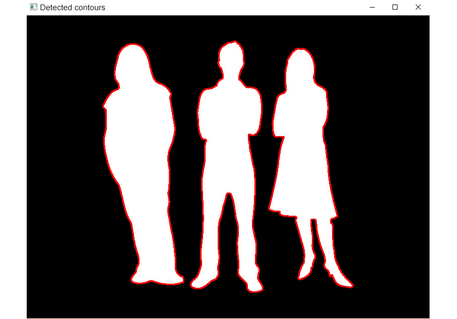
Figure 4.3: Contours drawn
In the next exercise, we will see how we can detect contours in a colored image.
Exercise 4.01: Detecting Shapes and Displaying Them on BGR Images
Let's say you have the following colored image with different shapes:
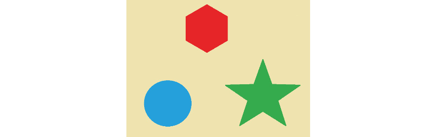
Figure 4.4: Image with shapes
Note
The image is also available at https://packt.live/2ZtOSQP.
Your task is to count all the shapes and detect their outer boundaries as follows:
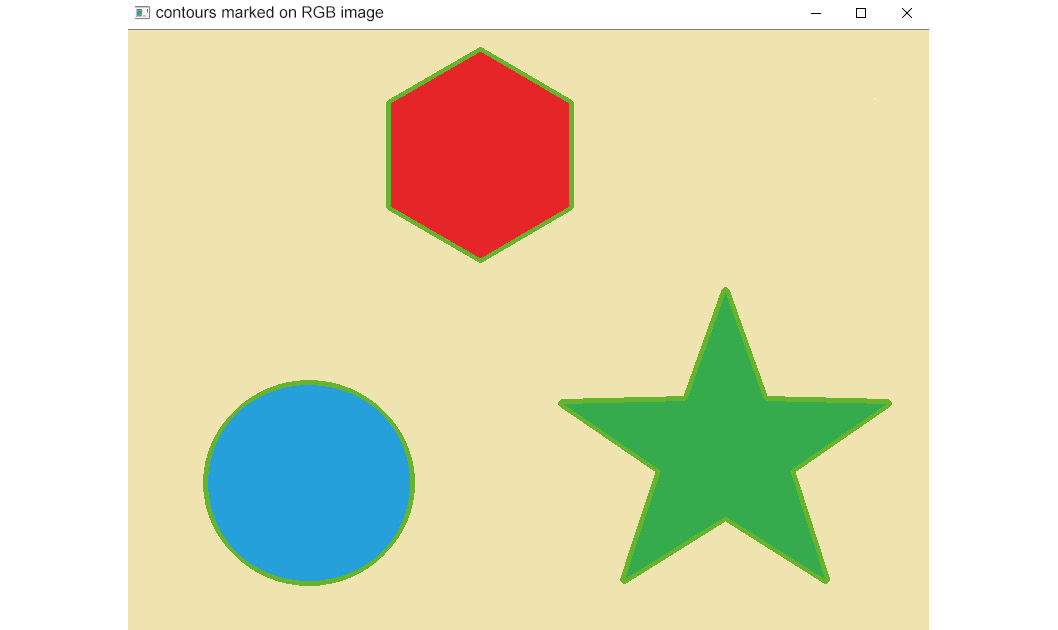
Figure 4.5: Required output
Perform the following steps:
- Open a new Jupyter notebook. Your working directory must contain the image file provided for this exercise. Click File | New File. A new file will open up in the editor. In the following steps, you will begin to write code in this file. Name the file Exercise4.01.
Note
The filename must start with an alphabetical character and must not have any spaces or special characters.
- Import OpenCV as follows:
import cv2
- Read the image as a BGR image:
image = cv2.imread('sample shapes.png')
- Convert it to grayscale:
gray_image = cv2.cvtColor(image, cv2.COLOR_BGR2GRAY)
- Now, display our grayscale image to see what it looks like. To display an image, we use the cv2.imshow command as in the following code. The first input to it is the text label that we want to caption our image with. The next input is the variable name that we have used for that image:
cv2.imshow('gray' , gray_image)
The output is as follows:
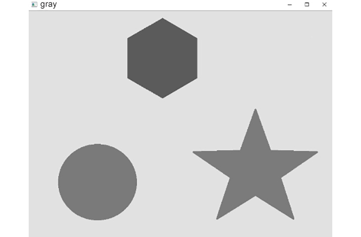
Figure 4.6: Grayscale image
The preceding command will display the image stored in the gray_image variable, with gray as the caption. However, the image will be displayed and all subsequent steps of the code will be brought to a standstill until you instruct your code on what to do next: that is, how long to wait before the program closes the image window and moves on.
- Add some code to have the image window wait until the user presses any key on the keyboard. For this instruction, we have the following command:
cv2.waitKey(0)
If you want to wait for a fixed length of time before closing the window, instead of having to wait for user input, you can use the cv2.waitKey(time_ms) command, where time_ms is the number of milliseconds you want the program to wait before automatically closing the window.
Now, our program will wait for the user to press any key on the keyboard and once our user presses it, the program execution will pass this line, so we need to give it the next instruction.
- Next, let's tell our program to close all open image windows before moving on to the next steps, using the following code:
cv2.destroyAllWindows()
- After this, we will now convert our image to binary. We are going to use Otsu's method to do this segmentation because it provides acceptable results for this image. In case Otsu's method does not give good results on your image, then you can always select a fixed threshold:
ret,binary_im = cv2.threshold(gray_image,0,255,
cv2.THRESH_OTSU)
cv2.imshow('binary image', binary_im)
cv2.waitKey(0)
cv2.destroyAllWindows()
The output is as follows:

Figure 4.7: Binary image
Now, before we apply contour detection to this image, let's analyze the objects we want to detect. We want to detect these black shapes on a white background. To apply OpenCV's implementation of contour detection here, first we need to make the background black and the foreground white. This is called inverting an image.
Note
In colored images, black is represented by 0 and white by 255. So, to invert it, we will simply apply the following formula: pixel= 255 – pixel. This is applied to the whole image as image= 255 – image.
In Python, an OpenCV image is stored as a NumPy array. Therefore, we can simply invert it as image= ~image.
Both commands give identical results.
- Next, invert the image and display it as follows:
inverted_binary_im= ~binary_im
cv2.imshow('inverse of binary image', inverted_binary_im)
cv2.waitKey(0)
cv2.destroyAllWindows()
The output is as follows:

Figure 4.8: Inverted binary image
- Find the contours in the binary image:
contours,hierarchy = cv2.findContours(inverted_binary_im,
cv2.RETR_TREE,
cv2.CHAIN_APPROX_SIMPLE)
- Now, mark all the detected contours on the original BGR image in any color (say, green). We will set the thickness to 3:
with_contours = cv2.drawContours(image, contours, -1,(0,255,0),3)
cv2.imshow('Detected contours on RGB image', with_contours)
cv2.waitKey(0)
cv2.destroyAllWindows()
The output is as follows:

Figure 4.9: Detected contours on an RGB image
Note
You can experiment with the value for thickness.
- Finally, display the total count of the detected contours:
print('Total number of detected contours is:')
print(len(contours))
The output is as follows:
Total number of detected contours is:
3
In this exercise, we practiced how to detect contours on a colored image. First, the image must be converted to grayscale and then to binary with a black background and a white foreground. After this, contours are detected and visualized on a BGR image using OpenCV functions.
Note
To access the source code for this specific section, please refer to https://packt.live/2CVdTg1.
Exercise 4.02: Detecting Shapes and Displaying Them on Black and White Images
In the preceding exercise, you plotted the contours on a colored image. Your next task is to plot the detected contours in a blue (BGR code: 255, 0, 0) color, but on the following black and white image:

Figure 4.10: Required output
Note
Complete steps 1 to 10 of Exercise 4.01, Detecting Shapes and Displaying Them on BGR Images, before you begin this exercise. Since this exercise is built on top of the previous one, it should be executed in the same Jupyter notebook.
- To draw contours with a BGR color code, the image must have three channels. So, we will replicate the single plane of the binary image three times and then merge the three planes to extend it into BGR color space. To merge the channels, refer the cv2.merge command you learned in the Important OpenCV Functions section of Chapter 1, Basics of Image Processing:
bgr = cv2.merge([inverted_binary_im,
inverted_binary_im, inverted_binary_im]);
- Now, mark all the detected contours on this generated BGR image in any color (say, blue). We will keep the thickness set to 3:
with_contours = cv2.drawContours(bgr, contours,
-1, (255,0, 0),3)
cv2.imshow('Detected contours', with_contours)
cv2.waitKey(0)
cv2.destroyAllWindows()
The output is as follows:

Figure 4.11: Detected contours on black and white images
Note
You can experiment with the value for line thickness.
In this exercise, we saw how contours can be drawn on a black and white image. Binary images have a single plane, whereas colored contours can only be drawn on an image with three planes, so, we will replicate the binary image to get three similar images (planes). These planes are merged to get an image in BGR format. After this, the detected contours are drawn on it.
Note
To access the source code for this specific section, please refer to https://packt.live/3eQyobZ.
Exercise 4.03: Displaying Different Contours with Different Colors and Thicknesses
This is an extension of the previous exercise. Having completed all the steps under Exercise 4.02, Detecting Shapes and Displaying Them on Black and White Images, we will do the following:
- Mark contour number 1 in red color with a thickness of 10.
- Mark contour number 2 in green color with a thickness of 20.
- Mark contour number 3 in blue color with a thickness of 30.
Note
This exercise is built on top of Exercise 4.02, Detecting Shapes and Displaying Them on Black and White Images and should be executed in the same Jupyter Notebook.
Perform the following steps:
- Take the BGR image stored in the bgr variable created in Step 1 of the previous exercise and draw contour #0 on it (that is, index 0 in the list of contours) in red (BGR code: 0, 0, 255). The thickness value will be 10. Let's call the output image (with the drawn contour) with_contours:
with_contours = cv2.drawContours(bgr, contours, 0,(0,0,255),10)
- Take the with_contours image and draw contour number 1 on it (that is, index 1 in the list of contours) in green (BGR code: 0, 255, 0). The thickness value will be 20. The with_contours image is updated in this step (the output image is given the same name as the input image):
with_contours = cv2.drawContours(with_contours, contours,
1,(0, 255, 0),20)
- Take the with_contours image and draw contour number 2 on it (that is, index 2 in the list of contours) in blue (BGR code: 255, 0, 0). The thickness value will be 30. The with_contours image is updated in this step as well:
with_contours = cv2.drawContours(with_contours, contours,
2, (255,0, 0), 30)
- Display the result using the following code:
cv2.imshow('Detected contours', with_contours)
cv2.waitKey(0)
cv2.destroyAllWindows()
The output is as follows:
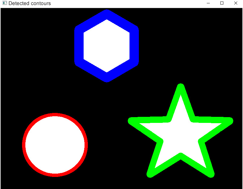
Figure 4.12: Final result
In this exercise, we practiced how to access individual contours from the list of detected contours. We also practiced giving different thicknesses and colors to the individual contours.
Note
To access the source code for this specific section, please refer to https://packt.live/2Zqfr9t.
Drawing a Bounding Box around a Contour
So far, you have learned how to draw the exact shape of the detected contours. Another important thing you might need to do in your projects is to draw an upright rectangular bounding box around your contours of interest.
For example, say you are asked to track a moving car in a video. The first thing you would do is to draw a bounding box around that car in all frames of the video. Similarly, face detection algorithms also draw bounding boxes around faces present in an image.
To draw a bounding box on any region of an image, you need the following:
- The starting x coordinate of the box
- The starting y coordinate of the box
- The width of the box (w)
- The height of the box (h)
You can get these parameters for a contour (around which you want to draw the bounding box) by passing that contour into the cv2.boundingRect function:
x, y, w, h= cv2.boundingRect(my_contour)
As an example, let's get these parameters for the first detected contour (which is the contour at index=0 in the list of contours) on the image in Figure 4.3:
x,y,w,h = cv2.boundingRect(contours[0])
The next step is to plot these values on the image. For this, we will use OpenCV's cv2.rectangle command:
cv2.rectangle(img,(x,y), (x+w,y+h), color_code, thickness)
This command takes as input the x and y coordinates in the top left of the image and the x and y coordinates in the bottom right of the image (with which we can compute the width and height). The color code and thickness values are also inputted according to the user's choice. Let's plot our box in blue with a thickness of 5:
cv2.rectangle(with_contours,(x,y), (x+w,y+h),
(255,0,0), 5)
cv2.imshow('contour#1', with_contours)
cv2.waitKey(0)
cv2.destroyAllWindows()
This will give you an output along the lines of the following:
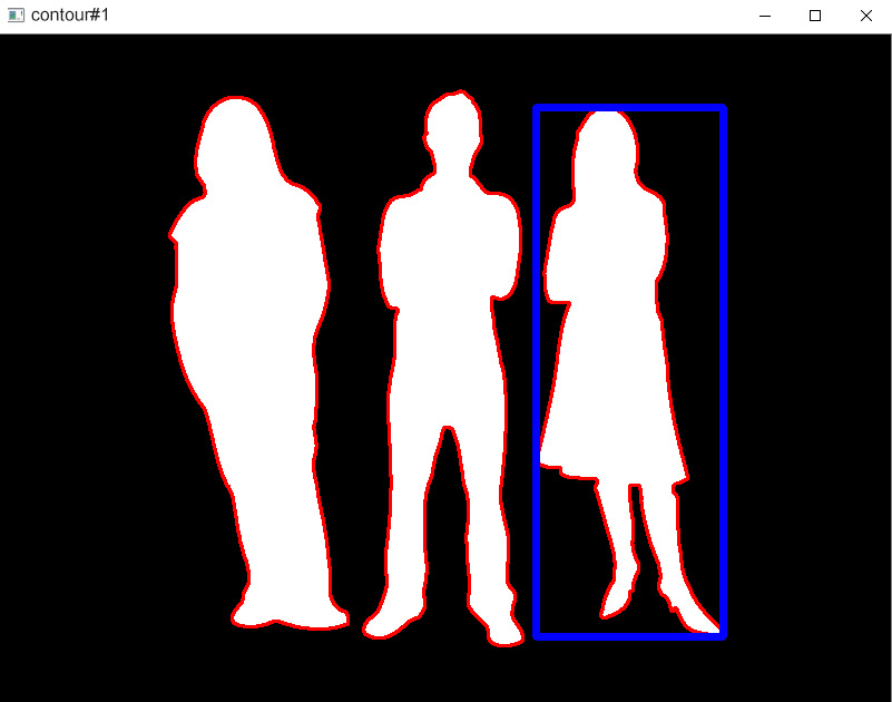
Figure 4.13: Contour number 1 enclosed in a blue bounding box
If you want to draw bounding boxes around all detected contours, then you should use a for loop. This for loop will iterate over all the contours and, for each detected contour, it will find x, y, w, and h and draw the rectangle over that contour.
Area of a Contour
OpenCV also provides you with some handy commands to get the attributes of a contour (including the area, the x and y coordinates of its centroid, the perimeter, the moments, and so on). You can visit https://docs.opencv.org/trunk/dd/d49/tutorial_py_contour_features.html for more details. One of the most commonly used attributes is the area of a contour. To get the area of a contour, you can use the following command:
contour_area = cv2.contourArea(contour)
You can also retrieve the contour with the maximum area as follows:
max_area_cnt = max(contour_list, key = cv2.contourArea)
Similarly, you can fetch the contour with the minimum area as follows:
min_area_cnt = min(contours, key = cv2.contourArea)
Difference between Contour Detection and Edge Detection
Looking at Figure 4.5, you may wonder that if these detections are of contours, then doesn't that make contour detection the same as edge detection? Not quite. At least not for images with subtle changes in intensity. According to the documentation relating to OpenCV, a contour is the boundary of an object whereas an edge is essentially the portion of an image with a significant change in intensity. For example, an object that has many different shades of color on its surface will have many distinct edges on its surface. But since it is one object, it will have only one boundary along its shape (contour).
For example, in the following image, have a close look at the surface of the banana:

Figure 4.14: Image of a banana
The intensity of color inside this banana varies significantly.
Contour detection will only give you the (closed) boundaries of the main object(s), whereas edge detection will give you all the detected regions where a change in intensity has taken place.
The results of contour detection are as follows:

Figure 4.15: Contour detection using the steps in the flowchart given in Figure 4.1
The results of performing edge detection on the sample image are as follows:
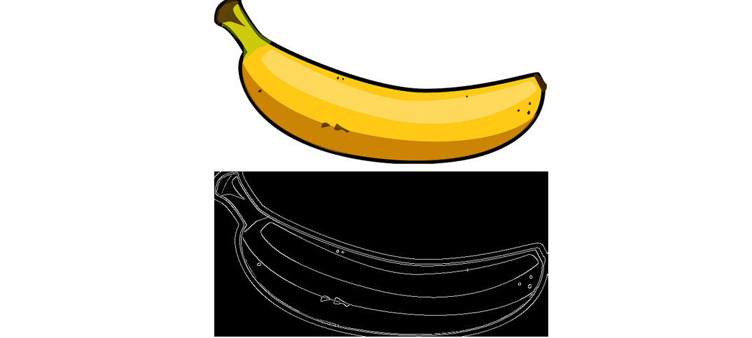
Figure 4.16: Edge detection
Edge detection for this sample banana image has marked all regions of the image where a change in intensity has occurred. Contour detection, on the other hand, gave us the outline of the shape according to the binary image generated. If you play around with different thresholds for binary conversion, you will get different binary images and, hence, different sets of contours.
You may observe that unlike edges, a contour is always a closed shape. In OpenCV, edge detection can directly be applied to an RGB image/grayscale image/binary image. Contour detection, on the other hand, is only for binary images.
Hierarchy
If you remember, in the Contours - Basic Detection and Plotting section, we saw that one of the inputs to the cv2.findContours function was named hierarchy. Now, what exactly is this thing? Well, contours can have relationships with one another. One contour might lie inside another larger contour – it will be the child of this larger contour. Similarly, a contour might even have grandchildren and great-grandchildren as well. These are called nested contours.
Let's look at the following diagram:

Figure 4.17: Total contours
How many contours do you see? 1, 2, or 3?
The answer is 3. Remember what we talked about at the start of this chapter. A contour is the boundary of a white object on a black background. The preceding image has a hollow square and a filled circle. You might be sure of the fact that the filled circle is a single blob; however, you might get confused with the hollow square. A hollow square has two outlines: the outer border, and the inner border; making two white borders and, hence, two contours on the square. That makes a total of three contours in the entire image:

Figure 4.18: Contours with hierarchy
To access the hierarchy information, you need to set the retrieval_mode input of cv2.findContours according to your requirements. When you learned about the cv2.findContours command at the start of this chapter, you saw the different input options (RETR_EXTERNAL, RETR_LIST, RETR_CCOMP, and RETR_TREE) for setting the contour retrieval mode.
Now, let's look at its corresponding output variable: hierarchy. If you take a look at the value of this hierarchy variable for any sample image, you will notice that it is a matrix with several rows equal to the number of detected contours. Consider the following contour retrieval commands and hierarchy structure for our sample image:

Figure 4.19: Contour retrieval commands and hierarchy structure for our sample image
Each row contains information about an individual contour. A row, as shown in the preceding figure, has four columns:
- column 1 contains the numeric ID of its next contour, which is on an identical hierarchical level. If such a contour does not exist, then its value here is listed as -1.
- column 2 contains the numeric ID of its previous contour, which is on an identical hierarchical level. If such a contour does not exist, then its value here is listed as -1.
- column 3 contains the numeric ID of its first child contour, which is at the next hierarchical level. If such a contour does not exist, then its value here is listed as -1.
- column 4 contains the numeric ID of its parent contour, which is at the next hierarchical level. If such a contour does not exist, then its value here is listed as -1.
Now, let's use these options on our sample image and see what happens. As a first step, let's read this sample image and save a copy.
Note
The sample image is available at https://packt.live/3etTonP.
Any changes made to the original image will not affect this copy. In the end, we can plot our results on this copy of the original image:
import cv2
image = cv2.imread('contour_hierarchy.png')
imagecopy= image.copy()
cv2.imshow('Original image', image)
cv2.waitKey(0)
cv2.destroyAllWindows()
The output is as follows:

Figure 4.20: Sample image
Such images are saved in a three-channel format. So, although this black and white image looks like a binary image, in reality, it is a three-channel BGR image. To apply contour detection to it, we would, of course, need to convert it to an actual single-channel binary image. We know that only grayscale images can be converted to binary.
We first need to convert the image to grayscale using the following code:
gray_image = cv2.cvtColor(image, cv2.COLOR_BGR2GRAY)
Note
In OpenCV, you can also read a BGR image directly as grayscale using the im = cv2.imread(filename,cv2.IMREAD_GRAYSCALE) command (note that the im = cv2.imread(filename,0) command will give identical results).
Now, we can convert it to binary:
ret, im_binary = cv2.threshold(gray_image, 00, 255, cv2.THRESH_BINARY)
The output is as follows:

Figure 4.21: Binary image
Now, let's go back to Figure 4.19. You can see that for cv2.RETR_EXTERNAL, there are only two detected contours. All inner contours are ignored.
The first row of its hierarchy matrix corresponds to contour 0. Its next contour is 1. Its previous contour does not exist (-1). Its child and parent contours also do not apply (-1 and -1) because only external contours are considered.
Similarly, the second row of its hierarchy matrix corresponds to contour 1. Its next contour does not exist (-1) because there are no more contours in this image. Its previous contour was contour 0. Its child and parent contours do not exist (-1 and -1 in the last two columns).
In Figure 4.19, for cv2.RETR_LIST, there are four detected contours. All inner contours are detected 'independently'. By 'independently' here, we mean that no parent-child relationship is formed (the last two columns are full of -1s). This means that all contours are considered to be at the same hierarchical level. There is a total of four contours in this image (since four rows are present). The first row has contour 0. It has contour 1 after it and no contour before it. The second row has contour 1. It has contour 2 after it and contour 0 before it. The third row has contour 2. It has contour 3 after it and contour 1 before it. The fourth row has contour 3. It has no contour after it (as there are no more contours left) and contour 2 before it.
For cv2.RETR_CCOMP, there are only two hierarchical levels. The outer boundaries of objects are on one level and the inner boundaries are on another level. Let's try to make sense of this hierarchy matrix here because it is not as simple as the first two. We know that a contour with only a single outer boundary (no hole) has no parent and no child. So, the last two columns for such a contour should be -1. The first two rows here have -1 in their last two columns – from this, we can gather that these first two rows correspond to the filled square and the filled circle. We also know that the first two columns give the indices of the next and previous contours on the same hierarchical level. If there is no other contour on the same level, then these two values should be -1, right? Look at the last row. It must belong to the inner hole of the hollow square because there is no other contour on that level (that is, there is no other inner hole boundary). That leaves us with row 3 and the outer boundary contour of the hollow square. So, row 3 must be for this contour. Do you want to confirm this? Well, this contour has a child contour but no parent contour, so for this contour, there would be a child but no parent, and this is reflected in the last two columns of row 3.
Finally, let's get to cv2.RETR_TREE. Look at the first row of its hierarchy matrix. Its last two columns have values of -1 and -1, so it is a contour with no child and no parent. Looking at the figure, we can easily conclude that it is a contour of the filled square. On the second row, we have a contour that has a child but no parent. So, it is the outer boundary of the hollow square. On the third row, we have a contour that has a child and a parent. So, it must be the boundary of the hole of the hollow square. In the last column, we have a contour that has no child but one parent. Hence, it must have no contours inside it, but a contour outside it. This explanation, of course, points to the filled circle in the center.
Exercise 4.04: Detecting a Bolt and a Nut
Suppose you are designing a system where a bolt is to be inserted into a nut. Using the image provided, you need to figure out the exact location of the following:
- The bolt, so that the robot can pick it up.
- The inner hole of the nut, so that the robot knows the exact location where the bolt is to be inserted.
Given the following binary image of the bolt and nut, detect the bolt and the inner hole of the nut:

Figure 4.22: Bolt and nut
Note
The image can be downloaded from https://packt.live/2YQWlKJ.
The bolt and the inner hole of the nut should be marked in separate colors as follows:
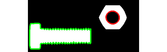
Figure 4.23: Required result
- Open a new file in Jupyter Notebook in the folder where the image file of the nut and bolt is present and save it as Exercise4.04.ipynb.
- Import OpenCV because this will be required for contour detection:
import cv2
- Read the three-channel black and white image:
image_3chan = cv2.imread('nut_bolt.png')
- Later, we are going to convert it into a single-channel binary image, so save a copy of this 3-channel image now to be able to plot the contours on it at the end of the exercise:
image_3chan_copy= image_3chan.copy()
- Display the original image:
cv2.imshow('Original image', image_3chan)
cv2.waitKey(0)
cv2.destroyAllWindows()
It will be displayed as follows:
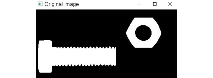
Figure 4.24: Original image of the nut and bolt
- Convert it to grayscale:
gray_image = cv2.cvtColor(image_3chan, cv2.COLOR_BGR2GRAY)
- Then, convert it to binary (using any suitable threshold) and display it as follows:
ret,binary_im = cv2.threshold(gray_image,250,255,cv2.THRESH_BINARY)
cv2.imshow('binary image', binary_im)
cv2.waitKey(0)
cv2.destroyAllWindows()
It will be displayed like this:

Figure 4.25: Binary image
In this binary image, we need to detect the outer boundary of the bolt and the inner boundary of the nut. Speaking in terms of hierarchy, the bolt is the only contour in this image that has no parent contour and no child contour. The inner hole of the nut, on the other hand, has a parent contour but no child contour. This is how we are going to differentiate between the two in the next steps.
- Find all contours in this image:
contours_list,hierarchy = cv2.findContours(binary_im,
cv2.RETR_TREE,
cv2.CHAIN_APPROX_SIMPLE)
We used RETR_TREE mode to get the contours because we are going to need their parent-child relationships.
- Let's print the hierarchy variable to see what it contains:
print('Hierarchy information of all contours:')
print (hierarchy)
The output is as follows:
Hierarchy information of all contours:
[[[ 1 -1 -1 -1]
[-1 0 2 -1]
[-1 -1 -1 1]]]
From here, we can see that this is a list containing one list inside it. This nested list is further made up of three lists. In the following diagram, you can see how to access the three individual lists:

Figure 4.26: Accessing the hierarchy of individual contours in the hierarchy variable
- In a for loop, we will now access the hierarchy information for each individual contour. For each contour, we will check the last two columns.
If both are -1, then that means that there is no parent and no child of that contour. This means that it is the contour of the bolt in the image. We will plot it in green to identify it.
If the third column is -1 but the fourth column is not -1, then that means that it has no child but does have a parent. This means that it is the contour of the inner hole of the nut in the image. We will plot it in red to identify it:
for i in range(0, len(contours_list)):
contour_info= hierarchy[0][i, :]
print('Hierarchy information of current contour:')
print(contour_info)
# no parent, no child
if contour_info[2]==-1 and contour_info[3]==-1:
with_contours = cv2.drawContours(image_3chan_copy,
contours_list,i,[0,255,0],thickness=3)
print('Bolt contour is detected')
if contour_info[2]==-1 and contour_info[3]!=-1:
with_contours = cv2.drawContours(with_contours,
contours_list,i,[0,0,255],thickness=3)
print('Hole of nut is detected')
The output is as follows:
Hierarchy information of current contour:
[ 1 -1 -1 -1]
Bolt contour is detected
Hierarchy information of current contour:
[-1 0 2 -1]
Hierarchy information of current contour:
[-1 -1 -1 1]
Hole of nut is detected
- Display the image with the marked contours:
cv2.imshow('Contours marked on RGB image', with_contours)
cv2.waitKey(0)
cv2.destroyAllWindows()
The preceding code will produce an output like this:

Figure 4.27: Bolt detected in green and the nut's hole in red
In this exercise, you implemented a practical example of accessing contours using their hierarchy information. This was meant to give you an idea of how the information stored in different contour retrieval modes can be useful in different scenarios.
Note
To access the source code for this specific section, please refer to https://packt.live/2CYL8iF.
In the next exercise, we will implement a scenario where you will detect the net of a basketball by selecting the largest contour in the image.
Exercise 4.05: Detecting a Basketball Net in an Image
Your task is to draw a bounding box around the basket after detecting it. The approach we will follow here is that we will convert this image to binary using such a threshold that the entire white region of the basket is detected as a single object. This will undoubtedly be the contour with the largest area here. Then, we will mark this largest contour with a bounding box. Here is the basketball.jpg image:

Figure 4.28: Image of a basketball net
Note
The image can be downloaded from https://packt.live/3ihLjpt.
The output should be something like this:
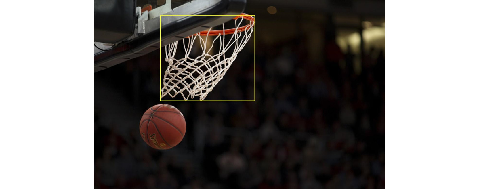
Figure 4.29: Required output
Let's perform the following steps to complete this exercise:
- Open Jupyter Notebook. Click on File | New File. A new file will open up in the editor. In the following steps, you will begin to write code in this file. Save the file by giving it any name you like.
Note
The name must start with an alphabetical character and must not contain any spaces or special characters.
- Jupyter Notebook requires us to import the necessary libraries and, for the current exercise, we will use OpenCV only. Import the OpenCV library using the following code:
import cv2
- Read the colored image using the following code:
image = cv2.imread('basketball.jpg')
- Make a copy of this image and save it to another variable using the following code:
imageCopy= image.copy()
This is just a safety precaution so that even if your original image is modified later in the code, you will have a copy saved in case you might need it later.
- Display the image you have read using the following code:
cv2.imshow('BGR image', image)
cv2.waitKey(0)
cv2.destroyAllWindows()
The output is as follows:

Figure 4.30: Input image
Press any key on the keyboard to close this image window and move forward.
- Convert the image to grayscale and display it as follows:
gray_image = cv2.cvtColor(image,cv2.COLOR_BGR2GRAY)
cv2.imshow('gray', gray_image)
cv2.waitKey(0)
cv2.destroyAllWindows()
Running the preceding code will produce the following output:

Figure 4.31: Grayscale image
- Convert this grayscale image to a binary image using a threshold such that the entire white boundary region of the basketball net is detected as a single blob:
ret,binary_im = cv2.threshold(gray_image,100, 255,
cv2.THRESH_BINARY)
cv2.imshow('binary', binary_im)
cv2.waitKey(0)
cv2.destroyAllWindows()
Using trial and error, we found 100 to be the best threshold, in this case, to convert the image to binary. If you find that some other threshold works better, feel free to use that.
Running the preceding code will display the following:

Figure 4.32: Binary image
- Detect all contours using the following code:
contours,hierarchy = cv2.findContours(binary_im,
cv2.RETR_TREE,cv2.CHAIN_APPROX_SIMPLE)
- Draw all the detected contours on the image and then display the image. Use the following code to plot all the contours in green:
contours_to_plot= -1
plotting_color= (0,255,0)
# if we want to fill the drawn contours with color
thickness= -1
with_contours = cv2.drawContours(image,contours, contours_to_plot,
plotting_color,thickness)
cv2.imshow('contours', with_contours)
cv2.waitKey(0)
cv2.destroyAllWindows()
A thickness of -1 was given to fill the drawn contours with color for a better visual display.
This will give you the following image output:

Figure 4.33: Drawn contours
- Next, we must plot bounding boxes around all contours. The code for this is given in the following snippet:
for cnt in contours:
x,y,w,h = cv2.boundingRect(cnt)
image = cv2.rectangle(image,(x,y),(x+w,y+h),
(0,255,255),2)
In the preceding code, we looped over each contour one by one and computed the starting x and y coordinates along with the width and height of a bounding box that would fit over each contour. Then, we plotted the identified rectangular bounding box for each contour on the actual image. We used yellow to draw the bounding boxes. The BGR code for yellow is (0, 255, 255). A thickness of 2 was used to draw the bounding boxes.
- Now, display the image using the following code:
cv2.imshow('contours', image)
cv2.waitKey(0)
cv2.destroyAllWindows()
This will give you the following image output:
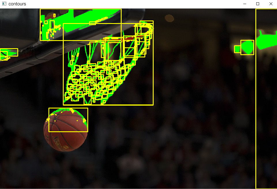
Figure 4.34: Detected contours bounding boxes around them
- Find the contour with the largest area:
required_contour = max(contours, key = cv2.contourArea)
- Find the starting x and y coordinates and the width and height of a rectangular bounding box that should enclose this largest contour:
x,y,w,h = cv2.boundingRect(required_contour)
- Draw this bounding box on a copy of the original colored image that you had saved earlier:
img_copy2 = cv2.rectangle(imageCopy, (x,y),(x+w, y+h),
(0,255,255),2)
- Now, display this image with the bounding box drawn over it:
cv2.imshow('largest contour', img_copy2)
cv2.waitKey(0)
cv2.destroyAllWindows()
This will give you the following output image:
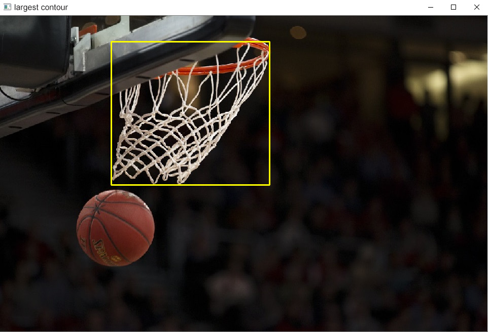
Figure 4.35: Final result
In this exercise, we learned how to apply contour detection to detect the net of a basketball hoop.
Note
To access the source code for this specific section, please refer to https://packt.live/31BlWJc.
In the next section, we are going to explore a method for finding the contour on an image that most closely matches a reference contour given in another image.
Contour Matching
In this section, we will learn how to numerically find the difference between the shapes of two different contours. This difference is found based on Hu moments. Hu moments (also known as Hu moment invariants) of a contour are seven numbers that describe the shape of a contour.
Note
Visit https://docs.opencv.org/2.4/modules/imgproc/doc/structural_analysis_and_shape_descriptors.html for more details.
Hu moments can be computed using OpenCV in the following way:
Image moments can be computed with the following command:
img_moments= cv2.moments(image)
The cv2.HuMoments OpenCV function is given the following moments as input:
hu_moments= cv2.HuMoments(img_moments)
This array is then flattened to get the feature vector for the Hu moments:
hu_moments= hu_moments.flatten()
This feature vector has a row with seven columns (seven numeric values).
Hu moment vectors of some sample contour shapes are shown in the following table:

Figure 4.36: Hu moment vectors of some sample contour shapes
For a Hu moment vector, consider the following:
- The first six values remain the same even if the image is transformed by reflection, translation, scaling, or rotation. What this means is that two contours of the same basic shape will have nearly equal values of these moments even if one of them is resized, rotated, flipped in any direction, or changes its position or location in the image (by way of an example, refer to the first six values in the last two rows of Figure 4.36).
- The seventh value changes sign (positive or negative) if the contour's image is flipped (for an example, refer to the last values in the last two rows of Figure 4.36).
Sounds interesting, doesn't it? Think of all the wonderful stuff you can do with it. Optical Character Recognition (OCR) is just the beginning.
The command to perform shape matching (the comparison of two shapes) using Hu moments is given in the following code. It will give you a numerical value describing how different the two shapes are from one another:
contour_difference = cv2.matchShapes (contour1, contour2,
compar_method, parameter)
The smaller the value of this output variable (contour_difference), the greater the similarity between the two compared contours. Concerning the aforementioned formula, note the following:
- contour1 and contour2 are the two individual contour objects you want to compare (alternatively, instead of giving contour objects, you can also give the cropped grayscale images of the two individual contours).
- compar_method is the method of comparison. It can either be an integer ranging from 1 to 3 or its corresponding string command, as outlined in the following table:

Figure 4.37: Three comparison methods of contours
You will find that cv.CONTOURS_MATCH_I1 works best in most scenarios. However, when working on a project, do test all three of these to see which one works best for your data.
- parameter is a value related to the chosen comparison method, but you don't need to worry about it because it has become redundant in the latest versions of OpenCV. Do note, however, that you might get an error if you don't pass in a fourth input to the cv2.matchShapes function. You can pass any number in its place and it would work just fine. Usually, we pass 0.
Let's compare the two contours as follows:

Figure 4.38: Contour 1 (binary_im1)
The second contour appears as follows:

Figure 4.39: Contour 2 (binary_im2)
If we want to find the numerical difference between them, then we can write the following command:
contour_difference = cv2.matchShapes (binary_im1,
binary_im2, 1, 0)
In the preceding code, binary_im1 is the image of contour 1, and binary_im2 is the image of contour 2.
If we execute this command, then the contour_difference output variable will tell us the difference in the Hu moment vectors of these two shapes using the CONTOURS_MATCH_I1 distance. It comes out as 0.1137 for this example.
In this section, you learned how to match shapes that can be described by a single blob. What if you want to match a symbol that has two blobs instead of one? For example, a question mark:

Figure 4.40: Sample question mark image
Look at Figure 4.40 of a question mark. It has two contours. If you want to find this symbol in an image, simple contour matching won't work. For that, you would use another similar technique called template matching. To read more about this, visit https://docs.opencv.org/2.4/doc/tutorials/imgproc/histograms/template_matching/template_matching.html.
Exercise 4.06: Detecting Fruits in an Image
You are given the following image of a selection of fruits:

Figure 4.41: Image of fruits
Your task is to detect all fruits present in this image. Do this via contour detection and draw the shapes of the contours on the image like so, such that the fruit contours are drawn in red:

Figure 4.42: Detected fruits
Note
The image is available at https://packt.live/3iinnSF.
Perform the following steps:
- Import the OpenCV library:
import cv2
- Now, read the image and display it as follows:
image = cv2.imread('many fruits.png')
cv2.imshow('Original image', image)
cv2.waitKey(0)
cv2.destroyAllWindows()
The preceding code produces the following output:

Figure 4.43: Original image
- Convert it to grayscale and display it as follows:
gray_image = cv2.cvtColor(image,cv2.COLOR_BGR2GRAY)
cv2.imshow('gray', gray_image)
cv2.waitKey(0)
cv2.destroyAllWindows()
The output is as follows:

Figure 4.44: Grayscale image
- Convert it to binary using a suitable threshold and display it. The threshold you select must give the outer boundaries of the fruits as single objects. It is okay if some holes remain in the middle of each fruit:
ret,binary_im = cv2.threshold(gray_image,245,
255,cv2.THRESH_BINARY)
cv2.imshow('binary', binary_im)
cv2.waitKey(0)
cv2.destroyAllWindows()
The output is as follows:

Figure 4.45: Binary image
- Since we require a white foreground on a black background to do contour detection in OpenCV, we will invert this image as follows:
binary_im= ~binary_im
cv2.imshow('inverted binary', binary_im)
cv2.waitKey(0)
cv2.destroyAllWindows()
The output is as follows:

Figure 4.46: Inverted binary image
Note that there are some empty pixels inside the fruits, so we will do external contour detection next.
- Find all the external contours as follows:
contours,hierarchy = cv2.findContours(binary_im,
cv2.RETR_EXTERNAL,cv2.CHAIN_APPROX_SIMPLE)
- Draw these contours in red on the original image and display it as follows:
with_contours = cv2.drawContours(image,contours,
-1,(0,0,255),3)
cv2.imshow('contours marked on RGB image', with_contours)
cv2.waitKey(0)
cv2.destroyAllWindows()
The output is as follows:

Figure 4.47: Detected external contours
In this exercise, you practiced contour detection by implementing the steps mentioned in the flowchart of Figure 4.1.
Note
To access the source code for this specific section, please refer to https://packt.live/3ggehUR.
Exercise 4.07: Identifying Bananas from the Image of Fruits
This exercise is an extension of Exercise 4.06, Detecting Fruits in an Image. You are given the following reference image containing a banana:

Figure 4.48: Reference image of a banana
Note
This exercise is built on top of the previous exercise and should be executed in the same notebook. The image is available at https://packt.live/2NLBPog.
Your task is to identify all bananas present in the image of the previous exercise and mark them in blue, as follows:

Figure 4.49: Required output
Perform the following steps:
- Read the reference image and display it using the following command:
ref_image = cv2.imread('bananaref.png')
cv2.imshow('Reference image', ref_image)
cv2.waitKey(0)
cv2.destroyAllWindows()
The output is as follows:

Figure 4.50: Reference image of a banana
- Convert it to grayscale and display the result as follows:
gray_image = cv2.cvtColor(ref_image,cv2.COLOR_BGR2GRAY)
cv2.imshow('Grayscale image', gray_image)
cv2.waitKey(0)
cv2.destroyAllWindows()
The output is as follows:

Figure 4.51: Grayscale version of the reference image
- Using a suitable threshold, convert it to binary and display the result:
ret,binary_im = cv2.threshold(gray_image,245,255,
cv2.THRESH_BINARY)
cv2.imshow('Binary image', binary_im)
cv2.waitKey(0)
cv2.destroyAllWindows()
The output is as follows:
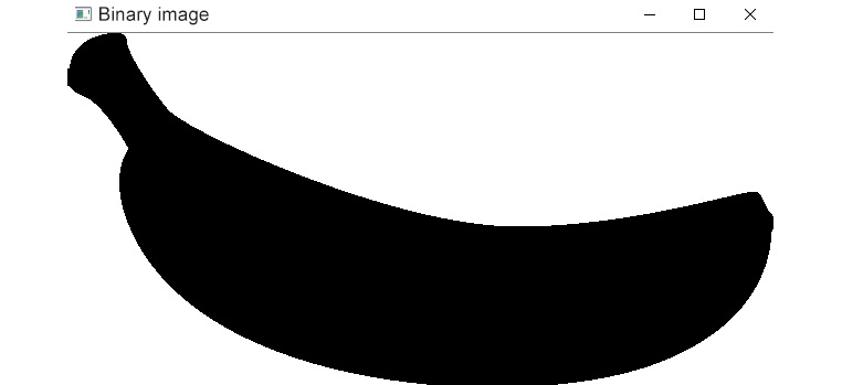
Figure 4.52: Binary version of the reference image
- To make the object white and the background black (which is required for the contour detection command in OpenCV), we will invert the image:
binary_im= ~binary_im
cv2.imshow('inverted binary image', binary_im)
cv2.waitKey(0)
cv2.destroyAllWindows()
The output is as follows:
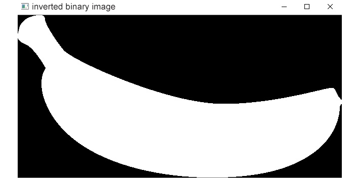
Figure 4.53: Inverted binary image
- Find the external boundary of this shape and draw a red outline on it:
ref_contour_list,hierarchy = cv2.findContours(binary_im,
cv2.RETR_EXTERNAL,
cv2.CHAIN_APPROX_SIMPLE)
with_contours = cv2.drawContours(ref_image,
ref_contour_list,-1,(0,0,255),3)
cv2.imshow('contours marked on RGB image',
with_contours)
cv2.waitKey(0)
cv2.destroyAllWindows()
The output is as follows:
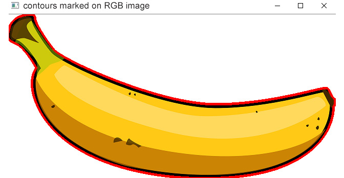
Figure 4.54: Detected contour in red
- There should only be one contour in this image – the contour of the banana. To confirm it, you can check the number of contours in the Python list, ref_contour_list, using the len(ref_contour_list)) command. You will find that there is only one contour present:
print('Total number of contours:')
print(len(ref_contour_list))
The output is as follows:
Total number of contours:
1
- Put this contour at index 0 of the list because it is the banana. It is also the only contour in this list:
reference_contour = ref_contour_list[0]
- Now, we have to compare each fruit contour we detected in the original image of the fruits with the reference contour of the banana. The for loop is the best way to go. Before starting the for loop, we will initialize an empty list by the name of dist_list. In each iteration of the for loop, we will append to it the numerical difference between the contour and the reference contour:
dist_list= [ ]
for cnt in contours:
retval=cv2.matchShapes(cnt, reference_contour,1,0)
dist_list.append(retval)
The next task is to find the two contours at the smallest distances from the reference contour.
- Make a copy of dist_list and store it in a separate variable:
sorted_list= dist_list.copy()
- Now, sort this list in ascending order:
sorted_list.sort()
Its first element now (sorted_list[0]) is the smallest distance and its second element (sorted_list[1]) is the second-largest distance – these two distances correspond to the two bananas present in the image.
- In the original dist_list list, find the indices where the smallest and second smallest distances are present:
# index of smallest distance
ind1_dist= dist_list.index(sorted_list[0])
# index of second smallest distance
ind2_dist= dist_list.index(sorted_list[1])
- Initialize a new empty list and append the contours at these two indices to it:
banana_cnts= [ ]
banana_cnts.append(contours[ind1_dist])
banana_cnts.append(contours[ind2_dist])
- Now, draw these two contours on the image in blue:
with_contours = cv2.drawContours(image, banana_cnts,
-1,(255,0,0),3)
cv2.imshow('contours marked on RGB image',
with_contours)
cv2.waitKey(0)
cv2.destroyAllWindows()
The output of the preceding code will be as follows:
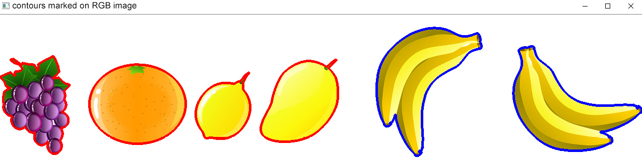
Figure 4.55: Detected bananas in blue
In this exercise, we implemented a scenario where we had to detect two bunches of bananas present in an image. A reference image of the banana was provided to allow us to do the matching. There was only a single banana present in the reference image, whereas in the image of all the fruits, there were two bunches of the bananas present. Each bunch had two bananas in it. One bunch was facing from left to right, whereas the other was in an upright position, yet contour matching detected them both successfully. This is because the shape of a bunch of two bananas is quite similar to the shape of a single banana. This exercise demonstrates the power of the contour-matching technique to retrieve similar-looking objects from an image.
Note
To access the source code for this specific section, please refer to https://packt.live/38gFN1H.
Exercise 4.08: Detecting an Upright Banana from the Image of Fruits
In this task, you will build on the work you did in the last exercise. In the previous exercise, you detected the two banana bunches in the image where multiple fruits were present. One bunch was in a horizontal position, and the other was in a vertical position. In this exercise, you will detect the banana bunch that is in an upright position as follows:

Figure 4.56: Required output
The task here is to draw a bounding box around that banana bunch whose height is greater than its width. Since this is an extension of the previous exercise, before proceeding with this, you must implement steps 1 to 13 of the previous exercise. After that, you can proceed as follows:
- Use a for loop to check each of these two contours one by one. If its height is greater than its width, plot a blue bounding box around it on the copy of the image you had saved earlier:
for cnt in banana_cnts:
x,y,w,h = cv2.boundingRect(cnt)
if h>w:
cv2.rectangle(imagecopy,(x,y),(x+w,y+h),
(255,0,0),2)
- Display this image:
cv2.imshow('Upright banana marked on RGB image', imagecopy)
cv2.waitKey(0)
cv2.destroyAllWindows()
The output is as follows:

Figure 4.57: Banana contour with height greater than the width
In this exercise, we put all our newly acquired skills to the test. We practically implemented the detection of contours, accessed them by hierarchy, did contour matching, and filtered the contours using their widths and heights. This should give you an idea of the many situations where contour detection and matching can come in handy.
Note
To access the source code for this specific section, please refer to https://packt.live/2Vw9MgU.
Activity 4.01: Identifying a Character on a Mirrored Document
When scanning documents, you know that you usually need to keep the paper steady, with the text in a straight horizontal orientation while the computer scans it. It would make for an interesting application to build a smart system that could read a document even if it is shown a mirror image or a lopsided image of it.
One of the basic tools you need for such an application is the ability to recognize a character even if it is inverted, flipped, mirrored, or slanted at an angle.
You are given two images. The first is of a rotated handwritten note that you captured through a mirror:
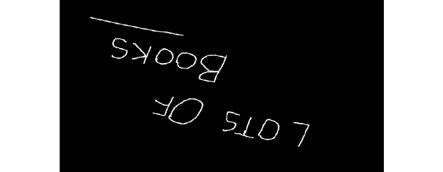
Figure 4.58: Handwritten note
Note
The image can be downloaded from https://packt.live/3ik9Lqc.
The second image is where you explicitly tell your program what the letter 'B' looks like. Your task is to write a program to identify where the letter 'B' occurs in the preceding image. You are given the following reference image for this:

Figure 4.59: Reference image for 'B'
Note
The image can be downloaded from https://packt.live/38hKDM1.
Your task here is to create a program that will identify where the letter 'B' occurs in the handwritten note, given the reference image of 'B' provided.
Your program should generate the following output:

Figure 4.60: Required output
Perform the following steps to complete the activity:
- Convert the reference image and the image of the handwritten note to binary form.
- Find all the contours on both these images using the cv2.RETR_EXTERNAL method.
- Compare each detected contour on the image of the handwritten note with the detected contour on the reference image to find the closest match.
- On the image of the handwritten note, mark the contour most similar to the contour on the reference image.
Note
The solution for this activity can be found on page 491.
In this activity, we learned how to apply contour detection to recognize the letter 'B'. The same technique can be applied to detect other alphabetical characters, digits, and special characters too – anything that can be represented as a single blob. Note that the 'B' in the reference image is written in quite a stylish, complex format. This is to demonstrate to you the strength of this technique of contour matching.
If you want to explore it further, you can make images with a handwritten 'B' or 'B' typed in some other standard formats and then take those as reference images instead. Print the minimum distance of the match and see how it varies for the following reference images:

Figure 4.61: Other possible reference images you can try
Summary
In this chapter, you learned that a contour is the outline of an object. This outline can either be on the outer border of the shape (an external contour) or it may be on a hole or other hollow surface inside the object (an inner contour). You learned how to detect contours of different objects and how to draw them on images using different colors. Also, you learned how to access different contours based on their area, width, and height.
Toward the end of the chapter, you gained hands-on experience of how to access the contours of a reference shape from an image containing multiple contours. This chapter can serve as a good foundation if you want to create smart systems, such as a license plate recognition system.
Up to Chapter 3, Working with Histograms, you learned about the basics of image processing using OpenCV. This chapter, on the other hand, was designed to give you a gentle push into the vast world of image processing and its practical applications in Computer Vision.
In the next chapter, you are going to learn how to detect a human face, the specific parts of a face, and even how to detect smiles in an image.