Overview
The objective of this chapter is to explain the concepts of object detection and facial recognition techniques and implement these techniques on input images or videos. The first part of this chapter addresses facial recognition techniques based on Eigenfaces, Fisherfaces, and Local Binary Pattern (LBP) methods. The second part focuses on object detection techniques, and it begins with a widely practiced method called MobileNet Single Shot Detector (SSD) and subsequently addresses the LBP and Haar Cascade algorithms. By the end of this chapter, you will be able to determine and implement the most suitable algorithms for object detection and facial recognition to solve practical problems.
Introduction
In the previous chapter, we learned how to implement various object tracking algorithms using the OpenCV library. Also, in Chapter 5, Face Processing in Image and Video, we discussed the concept of face detection. Now, it's time to discuss the next technique of face processing, called facial recognition. We will also discuss a few popular object detection techniques.
Facial recognition is a technique used to identify a person using their face in images or videos, including real-time image data. It is widely used by social media companies, companies manufacturing mobile devices, law enforcement agencies, and many others. One of the advantages of face recognition is that compared to other biometric processes, such as fingerprint or iris recognition, facial recognition is non-intrusive. It captures various facial features from an image and then analyzes and compares these features with facial features captured from other images to find the best match. In the first part of this chapter, we will discuss classical computer vision techniques used to implement facial recognition. It will provide a good foundation for you to start to explore more complex algorithms.
Object detection is a technique in which we aim to locate and identify all instances of objects (for example, people, vehicles, animals, and so on) present in a given image or video. It has many applications in the field of computer vision, such as pedestrian detection, vehicle detection, and ball tracking in sports.
Traditionally, object detection techniques were more reliant on feature engineering to find patterns in objects, and then these features would be used as an input to machine learning algorithms to locate objects. For example, suppose we needed to find a square-shaped box in an image. What used to happen is we would look for an object that has equal sides that are perpendicular to each other. Similarly, if another task was to find a face in an image, then we would look for features such as the distance between the eyes or the bridge of the nose (as with the Viola-Jones face detection algorithm). Since these approaches predominantly use rigidly engineered features, they often fail to generalize patterns of similar objects.
In 2012, the AlexNet architecture increased the accuracy of image classification tasks significantly in comparison to traditional methodologies, and this result led researchers to shift their focus to deep learning. With the advent of deep learning, the field of computer vision has seen great progress and improvement in the performance of object detection tasks. In the second part of this chapter, we will discuss traditional feature-based algorithms and deep learning algorithms (using OpenCV) for object detection.
We will start with face recognition, where we will discuss the Eigenface, Fisherface, and LBP methods for identifying faces. Then, we will discuss a deep learning algorithm called MobileNet SSD for object detection. Later on, we will discuss and implement the Local Binary Patterns Histograms (LBPH) method, a descriptor-based approach to detecting objects. In Chapter 5, Face Processing in Image and Video, we went through the concepts of Haar Cascade, so we will briefly revisit a few of the concepts and will conclude the discussion on object detection by applying the Haar Cascade method.
Face Recognition
Face recognition mainly involves the following stages:
- Pre-processing the images: Generally, when we work with unstructured data such as images, we are working with raw data. In the pre-processing step, we aim to improve the quality of the raw data either by removing any irregularities, such as distortions, non-alignments, and noise, or by enhancing some features using geometric transformation, such as zooming in, zooming out, translation, and rotation.
- Face detection: In this step, we aim to detect all the faces present in each image and store the faces with correct labels.
- Training (creating the face recognition model): In the training step, we take the images and their corresponding labels and feed them into a parametric algorithm that learns how to recognize a face. As a result, we get a trained parametric model that eventually helps us to recognize faces. The trained model contains some characteristic features corresponding to each unique label used during training.
- Face recognition: This step uses the trained model to verify whether the faces in two images belong to the same person. In other words, we pass an unknown image to the trained model, whereupon it extracts some characteristic features from that image and matches them with the features of training images and outputs the closest match.
The following figure depicts the preceding points:

Figure 7.1: Face recognition steps
In the preceding figure, the upper part represents the training step and the lower part represents the recognition step. Note that the sizes of the images in the left-most part of the figure are nearly the same (the size should be the same for algorithms such as Eigenface and Fisherface) as that of the images that come under the pre-processing step.
Note
The images used in Figure 7.1 are sourced from http://vis-www.cs.umass.edu/lfw/#download.
Face Recognition Using Eigenfaces
In this section, we will see how face recognition is achieved using Eigenfaces. Before diving into Eigenfaces, let's discuss an important concept in detail: dimensionality reduction and the Principal Component Analysis (PCA) technique.
Principal Component Analysis
Dimensionality reduction can be defined as a mapping of a higher-dimensional feature space (data points) to a lower-dimensional feature space, such that the maximum variance of the features remains intact. Principal component analysis, commonly known as PCA, is one of the more popular techniques used for dimensionality reduction. The objective of PCA is to identify the subspace in which the data can be approximated. In other words, the objective is to transform correlated features of large dimensions to the uncorrelated features of smaller dimensions.
Suppose we have a dataset of vehicles where each data point, x, has n different attributes (features); that is, x = x1, x2, xn. The attributes of the dataset can include speed in kph, speed in mph, engine capacity, size, and seating capacity. If we observe the attributes, we can see that the speed attributes are linearly dependent (meaning we can get speed in mph by applying some linear transformation to speed in kph) and hence are redundant. So, eventually, the dimension of the input features is n-1, not n.
Let's take another example. Suppose we have another dataset of football players with many attributes, such as salary, club, age, and skills (sliding tackle, standing tackle, and dribbling). Again, our goal is to reduce the dimensionality of the features such that we keep the more informative features and discard the less informative ones. Intuitively, we can say that if a player is good at sliding tackles, they may be good at standing tackles. So, these two features are correlated with each other. So, again, we may need a new single feature that represents these two original features, especially in regression analysis, which is used to understand and examine the relationship (usually a linear relationship, but it can be a higher degree polynomial relationship as well) between two variables, that is, a dependent variable and an independent variable.
The question that arises is this: how can we automatically detect redundant features? PCA helps to remove redundant features by transforming the original features of dimension n to new features of dimension d such that d<<n. The new feature dimensions are known as principal components, which are orthogonal (have no correlation) to each other and ordered in such a way that the variance of data decreases as we move down.
We can also see that PCA helps to represent images efficiently by discarding less informative features, eventually reducing complexity and memory requirements.
Eigenfaces
Eigenfaces can be defined as an appearance-based method that extracts the variation in facial images and uses this information to compare images of individual faces (holistic, not part-based) in databases. The Eigenfaces algorithm relies on the underlying assumption that not all facial details or features are equally significant. For example, when we see faces, we mainly notice prominent and distinct facial details, such as the nose, eyes, cheeks, or lips. In other words, we observe details that are distinct due to significant differences between facial features, such as the difference between a nose and an eye. Mathematically, this can be interpreted as the variance between those facial features being high. So, when we come across multiple faces, these distinct and important features help us to recognize people.
The Eigenfaces algorithm works in this way for facial recognition tasks. Its face recognizer takes training images and extracts the characteristics and features from those images, and then applies PCA to extract the principal components with maximum variance. We can refer to these principal components as Eigenfaces, or the eigenvectors of the covariance matrix of the set of images.
In the recognition phase, an unknown image is projected to the space formed by the Eigenfaces. Then, we evaluate a Euclidean distance between the eigenvectors of unknown images and the eigenvectors of the Eigenfaces. If the value of the Euclidean distance is small enough, then we tag that image with the most appropriate class. On the other hand, if we find that the Euclidean distance is large, then we infer that the individual's face was not present during the training phase and hence we model the images to accommodate the new image.
Note
The terms Eigenfaces and principal components will be used interchangeably in this chapter.
Until now, we have discussed the concepts of the Eigenfaces method. Now we will build a face recognizer using this method. Fortunately, OpenCV provides a facial recognition module called cv2.face.EigenFaceRecognizer_create(). We will use this facial recognition module to implement this exercise. We will feed the images of the respective classes to this module during the training phase and will use the trained model to recognize a new face.
This module mainly takes the following two parametric inputs:
- num_components: The number of components for PCA. There is no rule regarding how many components, but we aim for an amount that will maintain maximum variance. It also depends on the input data, so we can experiment with a few amounts.
- threshold: The threshold value is used while recognizing a new image. If the distance between the new image and its neighbor (another image used during training) is greater than the threshold value, then the model returns -1. This means that the model has failed to recognize the new image.
The following functions are used by the EigenFaceRecognizer module to train and test a model, respectively:
- eigenfaces_recognizer.train(): EigenFaceRecognizer uses this function to train a model using the training images. It takes the previously mentioned parameters as input arguments.
- eigenfaces_recognizer.predict(): EigenFaceRecognizer uses this function to predict the label of a new image. It takes a test image as an input argument.
Let's see the steps involved in the Eigenfaces algorithm. Figure 7.2 and Figure 7.3 depict the training steps and test steps for the Eigenfaces algorithm using OpenCV, respectively:

Figure 7.2: Training steps in the Eigenface algorithm
As shown in Figure 7.2, the training phase takes color or grayscale images as input. If the input is a color image, then the next step converts the input image into grayscale; otherwise, the input image is passed to the face detection function. As we discussed earlier, the Eigenface algorithm requires all images to be the same size; so, in the next step, all images are resized to the same dimensions. Then, the next step instantiates the recognizer model using the OpenCV module. After that, the model is trained using training images. The next figure shows the test steps in the Eigenfaces algorithm:
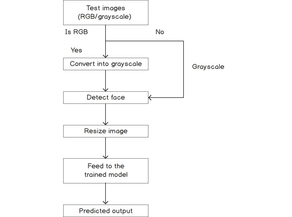
Figure 7.3: Steps during the test phase of the Eigenfaces algorithm
As shown in the preceding figure, the test phase first takes a new color or grayscale image as input. If the input is a color image, then the next step converts the input image into grayscale. Otherwise, the input image is passed to the face detection function. As we discussed earlier, the Eigenfaces algorithm requires all images to be the same size. Thus, in the next step, the test image is resized to the same size as the training images. Then, the next step feeds the resized image to the trained model (which was trained during the training steps), and finally outputs the category of the image.
Note
Before we go ahead and start working on the exercises and activities, please make sure that you have installed the opencv and opencv-contrib modules. If you are using Windows, it is recommended to use Anaconda. Please note that the code should be written in Python 3 or higher and the version of OpenCV should be 4 or higher.
Exercise 7.01: Facial Recognition Using Eigenfaces
In this exercise, you will be performing facial recognition using the Eigenfaces method. We will be using a training dataset to train the facial recognition model and a testing dataset to test the performance of the model. We will also be using Haar Cascades for face detection, which we studied in Chapter 5, Face Processing in Image and Video.
Note
The images used in this exercise are sourced from http://vis-www.cs.umass.edu/lfw/#download. Note that in this exercise, the faces of a few famous personalities have been used, but you can implement the exercise with any facial dataset.
Follow these steps to complete the exercise:
- Firstly, open an untitled Jupyter Notebook and name the file Exercise7.01.
- Start by importing all the required libraries for this exercise using the following code:
import cv2
import os
import numpy as np
import matplotlib.pyplot as plt
%matplotlib inline
- Next, specify the path of the dataset. Create a folder named dataset and, inside that, create two more folders: training-data and test-data. Put the training and test images into training-data and test-data, respectively.
Note
The training-data and test-data folders are available at https://packt.live/3dVDy5i.
The following code shows the path names and folder structure that needs to be maintained in your local system:
training_data_folder_path = 'dataset/training-data'
test_data_folder_path = 'dataset/test-data'
The structure of training-data looks as follows:
# directory of training data
dataset
training-data
|------0
| |--name_0001.jpg
| |--… …
| |--name_0020.jpg
|------1
| |--name_0001.jpg
| |--… …
| |-- name_0020.jpg
test-data
# similar structure
The idea is simple. The higher the number of images used in training, the better the result we will get from the model.
- Write the following code to check whether the images from the dataset are displayed properly:
random_image = cv2.imread('dataset/training-data'
'/1/Alvaro_Uribe_0020.jpg')
fig = plt.figure()
ax1 = fig.add_axes((0.1, 0.2, 0.8, 0.7))
ax1.set_title('Image from category 1')
plt.imshow(cv2.cvtColor(random_image, cv2.COLOR_BGR2RGB))
plt.show()
The above code produces the following output:

Figure 7.4: An image from the training dataset
The preceding code shows how to display an image from the dataset. Note that the folders titled 0,1,2 represent the image categories. The directory path should be in 'dataset/training-data/image_category/example_image.jpg' format, where example_image.jpg represents the filename. In the preceding code, the Alvaro_Uribe_0020.jpg image is displayed. To display images from another directory, just change the folder and image names to ones that correspond to your system setup.
- Now, specify the path of the OpenCV XML files that will be used to detect faces in each image. Create a folder named opencv_xml_files and save the haarcascade_frontalface.xml file inside that folder.
Note
The haarcascade_frontalface.xml file is available at https://packt.live/3gW5zeB.
The code is as follows:
haarcascade_frontalface = 'opencv_xml_files/
'haarcascade_frontalface.xml'
- Detect the face in the image using the detect_face function. This function first takes a color image as an input and converts it to grayscale. Then, it loads the XML cascade files that will detect faces in the image. Finally, it returns the faces and their coordinates in the input image:
def detect_face(input_img):
image = cv2.cvtColor(input_img, cv2.COLOR_BGR2GRAY)
face_cascade =
cv2.CascadeClassifier('opencv_xml_files'
'/haarcascade_frontalface.xml')
faces = face_cascade.detectMultiScale(image, scaleFactor=1.2,
minNeighbors=5)
if (len(faces)==0):
return -1, -1
(x, y, w, h) = faces[0]
return image[y:y+w, x:x+h], faces[0]
- Define a function named prepare_training_data. First, initialize two empty lists to store the detected faces and their respective categories. Read the images from the directories, as shown in step 3. Then, for each image, try to detect the faces. If a face is detected in the image, then resize the face to (121, 121) and append it to the list:
def prepare_training_data(training_data_folder_path):
detected_faces = []
face_labels = []
traning_image_dirs = os.listdir(training_data_folder_path)
for dir_name in traning_image_dirs:
label = int(dir_name)
training_image_path = training_data_folder_path + "/"
+ dir_name
training_images_names = os.listdir(training_image_path)
for image_name in training_images_names:
image_path = training_image_path + "/" + image_name
image = cv2.imread(image_path)
face, rect = detect_face(image)
if face is not -1:
resized_face = cv2.resize(face, (121,121),
interpolation = cv2.INTER_AREA)
detected_faces.append(resized_face)
face_labels.append(label)
return detected_faces, face_labels
Note
The Eigenfaces method expects all images to be the same size. To achieve that, we have fixed the dimensions of all images to (121,121). We can change this value. We can set the minimum size of the image as fixed dimensions or we can also take an average of dimensions.
- Use this code to call the function defined in the previous step:
detected_faces, face_labels = prepare_training_data(
"dataset/training-data")
- Print the number of training images and labels:
print("Total faces: ", len(detected_faces))
print("Total labels: ", len(face_labels))
The preceding code produces the following output:
Total faces: 105
Total labels: 105
Note that the number of training images and the number of labels should be equal.
- OpenCV is equipped with face recognizer modules. So, use the Eigenfaces recognizer module from OpenCV. Currently, the default parameter values are selected. You can specify the parameter values to see the result:
eigenfaces_recognizer = cv2.face.EigenFaceRecognizer_create()
You now have prepared the training data and initialized the face recognizer.
- Now, in this step, train the face recognizer model. Convert the labels into a NumPy array before passing it into the recognizer, as OpenCV expects labels to be a NumPy array:
eigenfaces_recognizer.train(detected_faces,np.array(face_labels))
- Define the draw_rectangle and draw_text functions. This will help to draw a rectangular box around the detected faces with the predicted class or category:
def draw_rectangle(test_image, rect):
(x, y, w, h) = rect
cv2.rectangle(test_image, (x, y), (x+w, y+h), (0, 255, 0), 2)
def draw_text(test_image, label_text, x, y):
cv2.putText(test_image, label_text, (x, y),
cv2.FONT_HERSHEY_PLAIN, 1.5, (0, 255, 0), 2)
- Let's predict the category of a new image. Define a function named predict that takes a new image as input. Then, it passes the image to the face detection function to detect faces in the test image. The Eigenface method expects an image of a certain size. So, the function will resize the test image to match the size of the training images. Then, in the next step, it passes the resized image to the face recognizer to identify the category of the image. The label_text variable will return the category of the image. Use the draw_rectangle function to draw a green rectangular box around the face using the four coordinates obtained during face detection. Alongside the rectangular box, the next line uses the draw_text function to write the predicted category of the image:
def predict(test_image):
detected_face, rect = detect_face(test_image)
resized_test_image = cv2.resize(detected_face, (121,121),
interpolation = cv2.INTER_AREA)
label = eigenfaces_recognizer.predict(resized_test_image)
label_text = tags[label[0]]
draw_rectangle(test_image, rect)
draw_text(test_image, label_text, rect[0], rect[1]-5)
return test_image, label_text
- Training images are made up of the following categories. These categories represent unique people to whom the faces that are detected belong. You can think of them as names corresponding to the faces:
tags = ['0', '1', '2', '3', '4']
- So far, you have trained the recognizer model. Now, you will test the model with test images. In this step, you will first read a test image.
Note
The image is available at https://packt.live/2Vv3uyb.
The code is as follows:
test_image = cv2.imread('dataset/test-data/1/Alvaro_Uribe_0021.jpg')
- Call the predict function to predict the category of the test image:
predicted_image, label = predict(test_image)
- Now, let's display the result of the test image. Step 16 returns the predicted image and the category label. Use matplotlib to display the images. Note that OpenCV generally represents RGB images in multi-dimensional arrays but in reverse order, that is, BGR. So, to display an image in the original order, use OpenCV's built-in cv2.COLOR_BGR2RGB function to convert BGR to RGB. Note that for each new test image, we must change the value of i in tags[i] to find out the actual class:
fig = plt.figure()
ax1 = fig.add_axes((0.1, 0.2, 0.8, 0.7))
ax1.set_title('actual class: ' + tags[1]+ ' | '
+ 'predicted class: ' + label)
plt.axis('off')
plt.imshow(cv2.cvtColor(predicted_image, cv2.COLOR_BGR2RGB))
plt.show()
The output is as follows:

Figure 7.5: Recognition result from the test data using the Eigenface method
You have predicted the category of a new image from class 1. Similarly, you can predict the category of different test images from other classes also.
Note
The test images of other classes are available at https://packt.live/38lUQaj.
To access the source code for this specific section, please refer to https://packt.live/2YN0ChZ.
In this exercise, you have learned how to implement a facial recognition model using the Eigenface method. You started off using Haar Cascade frontal face detection to detect the faces, and then you trained a facial recognition model using the training dataset. Finally, you used the testing dataset to find out about the performance of the model on an unseen dataset. You can also implement a similar model using a different dataset. You can extend the solution to retrieve similar images from the database.
But there are certain limitations to the Eigenfaces method. In the next section, we will discuss the limitations of this method, and then we will move on to look at the next method, called the Fisherface method.
Limitations of the Eigenface Method
We have discussed the underlying concepts of the Eigenface method and have implemented a face recognizer using Eigenfaces. But there are some limitations to this method. Before moving to the next method, let's discuss a few drawbacks of the Eigenface approach. We know that an Eigenface recognizer takes the facial features from all images at once and then it applies PCA to find the principal components (Eigenfaces). Intuitively, we can say that by considering all the features at once, we are not strictly capturing the distinct features of each image that would eventually help to distinguish between the faces of two different people.
Another drawback of this approach is that the effectiveness of PCA varies with illumination (lighting) levels. So, if we feed images with varying light levels to PCA, then the projected feature space will contain principal components that retain the maximum variation in lighting. It is possible that variation in the images due to the varying illumination levels may be greater than the variation due to the facial features of different people. Consequently, the recognition accuracy of an Eigenface recognizer will suffer.
For example, suppose we have images of people with varying illumination levels, as shown in Figure 7.6. Figure 7.6(a) shows the same face at varying illumination levels. Figure 7.6(b) and Figure 7.6(c) show two different people:

Figure 7.6: Faces of three different people
If we pass these images to an Eigenface face recognizer, then chances are high that PCA will give more importance to the faces shown in Figure 7.6(a) and may discard the features of faces shown in Figure 7.6(b) or Figure 7.6(c). Hence, an Eigenfaces face recognizer may not contain features of all the people and eventually will fail to recognize a few faces.
Variation due to illumination levels can be reduced by removing the 3 most significant principal components. But we do not know whether the three significant principal components are due to variation in lighting. So, the removal of the three significant features may lead to information loss.
We have discussed how facial recognition using Eigenfaces works. We have also gone through a few drawbacks. Now, we need to look for ways to improve the limitations of the Eigenfaces-based face recognizer and to do so, we will investigate another facial recognition technique called the Fisherfaces facial recognition method in the next section. We will see whether this method can solve the limitations of the Eigenface method.
Fisherface
In the previous section, we talked about how one of the limitations of the Eigenface method is that it captures the facial features of all the training images at once. We can solve this limitation if we extract the facial features of all the unique identities separately. So, even if there is variation in lighting, the facial features of one person will not dominate the facial features of others. The Fisherface method does this for us.
In facial recognition techniques, a low-dimensional feature representation with an enhanced discriminator function is always preferred. The Fisherface method uses Linear Discriminant Analysis (LDA) for dimensionality reduction. It aims to maximize inter-class separation and minimize separation within classes.
For example, suppose we have 10 unique identities, each with 10 faces. The Eigenface method will create 100 Eigenfaces corresponding to each image, but the Fisherface method will create 10 Fisherfaces corresponding to each class, not to each image. Consequently, variation inside one class will not affect other classes.
So, if PCA can perform dimensionality reduction, then why use LDA? We know that PCA aims to maximize the total variance in data. Though it is a widely practiced technique for representing data, it does not consider categories of data and eventually loses certain information. Due to this limitation, PCA fails under certain conditions.
LDA is also a dimensionality reduction technique, but LDA is a supervised method. It uses a label set during the training steps to build a more reliable dimensionality reduction method. Suppose we have two classes. LDA will compute the mean, μi, and variance, σi, of each class and project data points from the current feature dimensions to new dimensions such that it maximizes the difference between μ1 and μ2 and minimizes the variances, σ1 and σ2, within the class. Figure 7.7 shows how LDA dimensionality reduction works:

Figure 7.7: Dimensionality reduction in LDA
Let's look at an example to understand this. Suppose we have two-dimensional data as shown in Figure 7.7(a). Now, the aim of LDA is to find a line that will linearly separate the two-dimensional data, as shown in Figure 7.7(b). One way to do this could be projecting all the data points onto either one of the two axes, but this way, we will ignore information from the other axis. For example, if we project all the data points on the x axis, then we will lose information from the y axis. As discussed, LDA provides a better way. It projects the data points onto a new axis such that it maximizes the separation between the two categories, as shown in Figure 7.7(c) and Figure 7.7(d). Figure 7.7(e) shows the projected data on the new dimension.
So far, we have discussed the concepts of the Fisherface method. Now we will build a face recognizer using this method. Fortunately, OpenCV provides a face recognizer module called cv2.face.FisherFaceRecognizer_create(). We will use the Fisherface face recognizer module to implement the next exercise. We will feed images and their respective categories to this module during the training phase, and then we will use the trained model to recognize a new face.
This module takes two parameters. num_components is the number of components for LDA. Generally, we keep the number of components close to the number of categories. The default value for the number of components is c-1, where c represents the number of categories. So, if we don't provide a number, it is automatically set to c-1. If we provide a value less than 0 or greater than c-1, it will be set to the default. The other parameter is value.threshold. Refer to the threshold part of the Eigenfaces section of this chapter.
The following functions are used by the FisherFaceRecognizer module to train and test a model respectively:
- fisherfaces_recognizer.train(): This function is used to train the model. It takes the previously mentioned parameters as input arguments.
- fisherfaces_recognizer.predict(): This function is used to predict the label of a new image. It takes an image as an input argument.
We have discussed the underlying concepts of LDA. Let's discuss the major steps of the Fisherface method in face recognition. Figure 7.8 and Figure 7.9 depict the training steps and test steps of the Fisherface algorithm using OpenCV, respectively:

Figure 7.8: Training steps of the Fisherface algorithm
As shown in Figure 7.8, the training starts with taking a color or grayscale image as input. If the input is a color image, then the next step converts the input image into grayscale; otherwise, the input image is passed to the face detection function. As we discussed earlier, the Fisherface algorithm requires images to be of the same size; hence, in the next step, all images are resized to the same dimensions. Then, the next step instantiates the recognizer model using the OpenCV module. Finally, the model is trained using the training images:
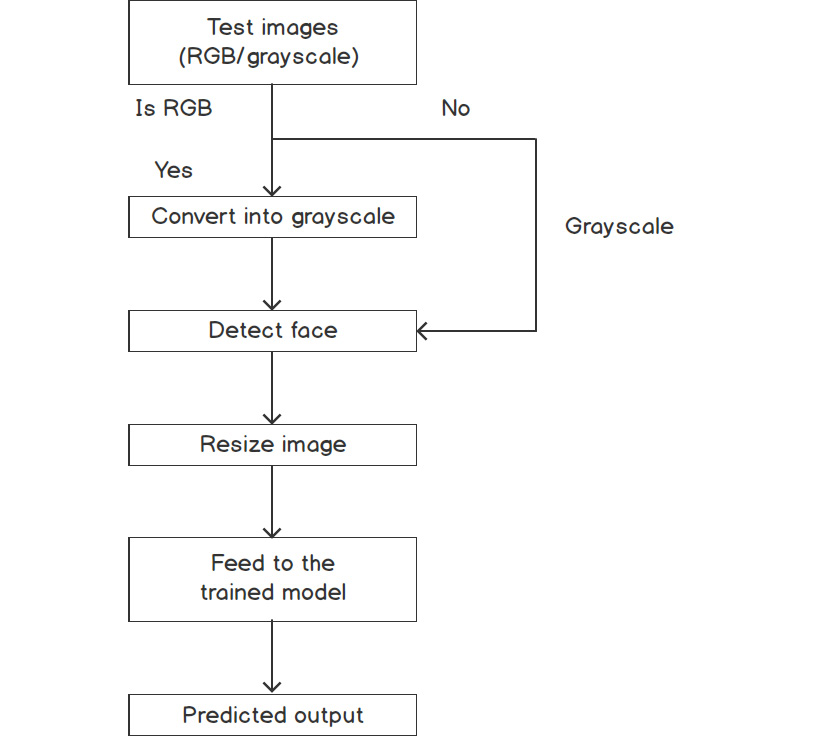
Figure 7.9: Steps during the test phase of the Fisherface algorithm
As shown in Figure 7.9, the testing starts with the model taking a new color or grayscale image as input. If the input is a color image, then the next step converts the input image into grayscale; otherwise, the input image is passed to the face detection function. As we discussed earlier, the Fisherface algorithm requires images to be of the same size; hence, in the next step, all images are resized to the same dimensions. Then, the next step feeds the resized image to the trained model (which was trained during the training steps), and, finally, it outputs the category of the input image.
Exercise 7.02: Facial Recognition Using the Fisherface Method
In this exercise, we will be performing facial recognition using the Fisherface method. The images used in this exercise are sourced from http://vis-www.cs.umass.edu/lfw/#download. Note that in this exercise, the faces of a few famous personalities have been used, but you can implement the exercise with any facial dataset. For this exercise, the basic pipeline will stay the same as in Exercise 7.01, Facial Recognition Using Eigenfaces. We will start by using Haar Cascades for frontal face detection and then the Fisherface method for face recognition:
- Firstly, open an untitled Jupyter Notebook and name the file Exercise7.02.
- Import all the required libraries for this exercise:
import cv2
import os
import numpy as np
import matplotlib.pyplot as plt
%matplotlib inline
- Next, specify the path of the dataset. Create a folder named dataset and, inside that, create two more folders, training-data and test-data. Put the training and test images in training-data and testing-data, respectively.
Note
The training-data and test-data folders are available at https://packt.live/2WibmU4.
The code is as follows:
training_data_folder_path = 'dataset/training-data'
test_data_folder_path = 'dataset/test-data'
- Display a training sample using matplotlib. To check whether the images from the dataset are being displayed correctly, use the following code:
random_image = cv2.imread('dataset/training-
data/2/George_Robertson_0020.jpg')
fig = plt.figure()
ax1 = fig.add_axes((0.1, 0.2, 0.8, 0.7))
ax1.set_title('Image from category 2')
# change category name #accordingly
plt.imshow(cv2.cvtColor(random_image, cv2.COLOR_BGR2RGB))
plt.show()
The output is as follows:

Figure 7.10: An image from the training dataset
The preceding code shows how to display an image from the dataset. Note that the folders titled 0,1,2 represent the image categories. The directory path should be in 'dataset/training-data/image_category/example_image.jpg' format, where example_image.jpg represents the filename. In the preceding code, the image titled George_Robertson_0020.jpg is displayed. To display images from another directory, just change the folder and image names to ones that correspond to your system setup.
- Specify the path of the OpenCV XML files that will be used to detect faces in each image. Create a folder named opencv_xml_files and save haarcascade_frontalface.xml inside that folder.
Note
The haarcascade_frontalface.xml file is available at https://packt.live/38fDThI.
The code is as follows:
haarcascade_frontalface = 'opencv_xml_files/ haarcascade_frontalface.xml'
- Detect the faces in an image using the detect_face function. This function takes color images as input and converts them to grayscale. Then, it loads the XML cascade files that will detect faces in the image. Finally, it returns the faces and their coordinates in the input image:
def detect_face(input_img):
image = cv2.cvtColor(input_img, cv2.COLOR_BGR2GRAY)
face_cascade = cv2.CascadeClassifier(
haarcascade_frontalface)
faces = face_cascade.detectMultiScale(image,
scaleFactor=1.2, minNeighbors=5);
if (len(faces)==0):
return -1, -1
(x, y, w, h) = faces[0]
return image[y:y+w, x:x+h], faces[0]
- Define the prepare_training_data function. This will first initialize two empty lists that will store the detected faces and their respective categories. Then it reads images from directories, shown in Step 3. Then, for each image, it tries to detect faces. If a face is detected in the image, then it resizes the face to (121, 121) and appends it to the list:
def prepare_training_data(trainig_data_folder_path):
detected_faces = []
face_labels = []
traning_image_dirs = os.listdir(training_data_folder_path)
for dir_name in traning_image_dirs:
label = int(dir_name)
training_image_path = training_data_folder_path +
"/" + dir_name
training_images_names = os.listdir(training_image_path)
for image_name in training_images_names:
image_path = training_image_path + "/" + image_name
image = cv2.imread(image_path)
face, rect = detect_face(image)
if face is not -1:
resized_face = cv2.resize(face, (121,121),
interpolation = cv2.INTER_AREA)
detected_faces.append(resized_face)
face_labels.append(label)
return detected_faces, face_labels
Note
The Fisherface method expects all images to be of the same size. To achieve that, we have fixed the dimensions of all images at (121,121). We can change this value. We can set the minimum size of the image or we can also take an average of the dimensions.
- Call the function mentioned in the previous step:
detected_faces, face_labels =
prepare_training_data("dataset/training-data")
- Display the number of training images and labels:
print("Total faces: ", len(detected_faces))
print("Total labels: ", len(face_labels))
The preceding code produces the following output:
Total faces: 105
Total labels: 105
- Use the Fisherface recognizer module from OpenCV. Currently, the default value of the parameter is selected:
fisherfaces_recognizer = cv2.face.FisherFaceRecognizer_create()
- You have prepared the training data and initialized a face recognizer. Now, in this step, train the face recognizer. Note that the labels are first converted into a NumPy array before being passed to the recognizer because OpenCV expects labels to be a NumPy array:
fisherfaces_recognizer.train(detected_faces, np.array(face_labels))
- Define the draw_rectangle and draw_text functions. These help to draw rectangular boxes around detected faces with the predicted class or category:
def draw_rectangle(test_image, rect):
(x, y, w, h) = rect
cv2.rectangle(test_image, (x, y), (x+w, y+h),
(0, 255, 0), 2)
def draw_text(test_image, label_text, x, y):
cv2.putText(test_image, label_text, (x, y),
cv2.FONT_HERSHEY_PLAIN, 1.5, (0,255, 0), 2)
- Now, let's predict the category of a new image. The predict function takes a new image as input. Then, it passes the image to the face detection function to detect faces in the test image. As discussed earlier, the Fisherface method expects a fixed-size image. So, the function will resize the test image to match the size of the training images. Then, in the next step, it passes the resized image to the face recognizer to identify the category of the image. The label_text variable will return the category of the image. Finally, it uses the draw_rectangle function to draw a green rectangular box around the face using the four coordinates obtained during face detection. Alongside the rectangular box, the next line uses the draw_text function to write the predicted category of the image:
def predict(test_image):
detected_face, rect = detect_face(test_image)
resized_face = cv2.resize(detected_face, (121,121),
interpolation = cv2.INTER_AREA)
label = fisherfaces_recognizer.predict(resized_face)
label_text = tags[label[0]]
draw_rectangle(test_image, rect)
draw_text(test_image, label_text, rect[0], rect[1]-5)
return test_image, label_text
- The training images have the following categories. This is similar to the tags array we used in the previous exercise. The basic idea behind using these tags is to show that the faces belong to a specific category/class:
tags = ['0', '1', '2', '3', '4']
- Then, we need to test the model with the test images. In this step, the test image is read and converted to grayscale:
Note
The image is available at https://packt.live/2Zsw3ig.
test_image = cv2.imread('dataset/test-data/2/
George_Robertson_0021.jpg')
- Call the predict function to predict the category of the test image:
predicted_image, label = predict(test_image)
- Finally, let's display the result of the test image. Step 16 returns the predicted image and its respective category label. Use matplotlib to display the images. Note that OpenCV generally represents RGB images in multi-dimensional arrays, but in reverse order, that is, BGR. So, to display the images in the original order, we will use OpenCV's built-in cv2.COLOR_BGR2RGB function to convert from BGR to RGB. Figure 7.11 shows the prediction results:
fig = plt.figure()
ax1 = fig.add_axes((0.1, 0.2, 0.8, 0.7))
ax1.set_title('actual class: ' + tags[2]+ ' | '
+ 'predicted class: ' + label)
plt.axis('off')
plt.imshow(cv2.cvtColor(predicted_image, cv2.COLOR_BGR2RGB))
plt.show()
The output is as follows:

Figure 7.11: Recognition result on test data using the Fisherface method
In this exercise, you have predicted the category of a new image from class 2. Similarly, you can predict the categories of different test images from other classes also. We also learned how we can use the Fisherface method for face recognition. One important thing to note here is the ease with which you can shift from the Eigenface recognition method to the Fisherface method by just changing one OpenCV function.
Note
The test images of other classes are available at https://packt.live/3gf6hDr.
To access the source code for this specific section, please refer to https://packt.live/38f3ibx.
Now we know that the Fisherface method helps to capture the facial features of all the unique identities separately. So, the facial features of one person will not dominate the others. Despite this, the method still considers varying illumination levels as a feature. We know that illumination changes create incoherence in images, and consequently, the performance of a face recognizer reduces. In the next section, we will discuss another facial recognition algorithm and find out whether it solves the illumination problem.
Local Binary Patterns Histograms
We have talked about how the Eigenface and Fisherface methods consider illumination changes as features. We also know that it is not always possible to have ideal lighting conditions. So, we need a method that addresses the limitation of varying illumination. The LBPH method helps to overcome that limitation.
The LBPH algorithm uses a local image descriptor called Linear Binary Pattern (LBP). LBP describes the contrast information of a pixel with regard to its neighboring pixels. It describes each pixel in an image with a certain binary pattern. It generally applies to grayscale images. The LBP method does not consider a complete image at once. Instead, it focuses on the local structure (patches) of an image by comparing each pixel to its neighboring pixels.
Let's discuss how LBP extracts features from an image. Originally, LBP was defined for a window (filter) of size 3x3, as shown in Figure 7.12(a), but a circular LBP operator can be used to improve performance, shown in Figure 7.12(b). Generally, it takes the center pixel's value as the threshold value for the window and compares this threshold with its neighboring 8 pixels. We can also consider the average pixel value as a threshold:
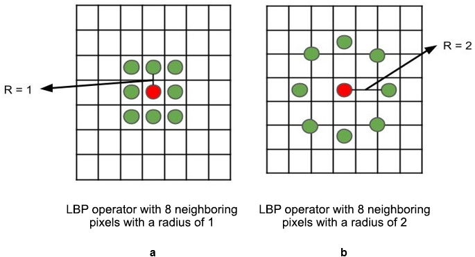
Figure 7.12: LBP operators with radii of 1 and 2
Now, if the values of adjacent pixels are greater than or equal to the threshold value, then you substitute the pixel value with 1; otherwise, you substitute it with 0, as shown in Figure 7.13. As a result, this generates an 8-bit binary number that is then converted to a decimal number to obtain the LBP value of the center pixel:

Figure 7.13: Estimation of LBP values
This LBP value is considered as the textual features of that local region. The LBP operator computes the LBP value for each pixel of an image. After calculating the LBP values for each pixel, the LBPH method converts those values into a histogram. Eventually, we will have a histogram for each image in the dataset. So, LBPH uses a combination of LBP and histograms to represent the feature vectors of an image. Note that this local features-based approach provides more robustness against illumination changes.
Until now, we have discussed the underlying concepts of the LBPH method. Now we will build a face recognizer using this method. We will use the LBPH face recognizer module called cv2.face.LBPHFaceRecognizer_create() from OpenCV to implement the next exercise. We will feed the images and their respective categories to this module during the training phase, and we will use the trained model to recognize a new face. We will mainly be concerned with three input parameters for this module:
- radius: As shown in Figure 7.12(b), the LBPH method can also build circular local binary patterns. The parameter radius determines the positions of adjacent pixels.
- neighbors: The number of adjacent pixels to determine the LBP value. We can also create more adjacent pixels using interpolation methods such as bilinear interpolation. Note that the computational cost is proportionate to the number of adjacent pixels.
- threshold: Refer to the threshold part of the Eigenfaces section of this chapter.
The following functions are used by the LBPHFaceRecognizer module to train and test a model respectively:
- lbphfaces_recognizer.train(): This function is used to train the model. It takes the previously mentioned parameters as input arguments.
- lbphfaces_recognizer.predict(): This function is used to predict the label of a new image. It takes an image as its input argument.
Let's discuss the major steps involved in the LBPH algorithm. Figure 7.14 and Figure 7.15 depict the training steps and test steps in the LBPH algorithm using OpenCV, respectively:

Figure 7.14: Training steps of the LBPH algorithm
As shown in Figure 7.14, the training steps first take color or grayscale images as input. If the input is a color image, then the next step converts the input image into grayscale; otherwise, the input image is passed to the face detection function. The LBP algorithm does not necessarily require images to be the same size; hence, a resize function will not be implemented in the next exercise. Then, the next step instantiates the recognizer model using the OpenCV module. Finally, the model is trained using training images:

Figure 7.15: Steps during the test phase of the LBPH algorithm
As shown in Figure 7.15, the testing starts with a new color or grayscale image being taken as input. If the input is a color image, then the next step converts the input image into grayscale; otherwise, the input image is passed to the face detection function. The LBP algorithm does not necessarily require images to be of the same size; hence, a resize function will not be implemented in the next exercise. Then, the next step feeds the image to the trained model (which was trained during training steps). Finally, it outputs the category of the input image.
Exercise 7.03: Facial Recognition Using the LBPH Method
In this exercise, we will be performing facial recognition using the LBPH method. The problem statement and the dataset will stay the same as those for the previous two exercises. We will only be changing the facial recognition method being used. This way, you will get hands-on experience of using different techniques for facial recognition:
- Firstly, open an untitled Jupyter Notebook and name the file Exercise7.03 or face_recongition_lbph.
- Start by importing all the required libraries for this activity:
import cv2
import os
import numpy as np
import matplotlib.pyplot as plt
%matplotlib inline
- Then, specify the path of the dataset. Create a folder named dataset and, inside that, create two more folders, training-data and test-data. Put the training and test images into training-data and test-data, respectively.
Note
The training-data and test-data folders are available at https://packt.live/3eFDsPr.
The code is as follows:
training_data_folder_path = 'dataset/training-data'
test_data_folder_path = 'dataset/test-data'
- Display a training sample using matplotlib. To check whether the images from the dataset are displaying correctly, use the following code:
random_image = cv2.imread('dataset/training-data/3
/George_W_Bush_0020.jpg')
fig = plt.figure()
ax1 = fig.add_axes((0.1, 0.2, 0.8, 0.7))
ax1.set_title('Image from category 3')
# change category name accordingly
plt.imshow(cv2.cvtColor(random_image, cv2.COLOR_BGR2RGB))
plt.show()
The output is as follows:

Figure 7.16: An image from the training dataset
In the preceding code, the image titled George_W_Bush_0020.jpg is displayed. To display images from another directory, just replace the folder and image names with any other existing folder and image names.
- Specify the path of the OpenCV XML files that will be used to detect the faces in each image. Create a folder named opencv_xml_files and save lbpcascade_frontalface.xml inside that folder. Instead of haarcascade, this time we will use lbpcascade, for LBP-based face detection:
lbpcascade_frontalface = 'opencv_xml_files/lbpcascade_frontalface.xml'
Note
The lbpcascade_frontalface.xml file is available at https://packt.live/2CTmHD3.
- Use the detect_face function to detect the faces in an image. It first takes a color image as an input and converts it to grayscale. Then, it loads the XML cascade files that will detect the faces in the image. Finally, it returns the faces and their coordinates in the input image:
def detect_face(input_img):
image = cv2.cvtColor(input_img, cv2.COLOR_BGR2GRAY)
face_cascade = cv2.CascadeClassifier(lbpcascase_frontalface)
faces = face_cascade.detectMultiScale(image,
scaleFactor=1.2, minNeighbors=5)
if (len(faces)==0):
return -1, -1
(x, y, w, h) = faces[0]
return image[y:y+w, x:x+h], faces[0]
- Define the prepare_training_data function such that it first initializes two empty lists that will store the detected faces and their respective categories, which will be eventually used for the training. Then, it should read the images from the directories shown in Step 3. Then, from each image, it tries to detect faces. If a face is detected in the image, then it appends the image to the list:
def prepare_training_data(training_data_folder_path):
detected_faces = []
face_labels = []
traning_image_dirs = os.listdir(training_data_folder_path)
for dir_name in traning_image_dirs:
label = int(dir_name)
training_image_path = training_data_folder_path +
"/" + dir_name
training_images_names = os.listdir(training_image_path)
for image_name in training_images_names:
image_path = training_image_path + "/" + image_name
image = cv2.imread(image_path)
face, rect = detect_face(image)
if face is not -1:
resized_face = cv2.resize(face, (121,121),
interpolation = cv2.INTER_AREA)
detected_faces.append(resized_face)
face_labels.append(label)
return detected_faces, face_labels
Note
The LBPH method does not expect all the training images to be of the same size.
- Call the function mentioned in the previous step:
detected_faces, face_labels = prepare_training_data("dataset/training-data")
- Display the number of training images and labels:
print("Total faces: ", len(detected_faces))
print("Total labels: ", len(face_labels))
The preceding code produces the following output:
Total faces: 93
Total labels: 93
- OpenCV is equipped with face recognizer modules. Use the LBPHFaceRecognizer module from OpenCV:
lbphfaces_recognizer =
cv2.face.LBPHFaceRecognizer_create(radius=1, neighbors=8)
- In the previous two steps, we have prepared the training data and initialized a face recognizer. Now, in this step, we will train the face recognizer. Note that the labels are first converted into a NumPy array before being passed into the recognizer because OpenCV expects labels to be a NumPy array:
lbphfaces_recognizer.train(detected_faces, np.array(face_labels))
- Define the draw_rectangle and draw_text functions. This helps to draw rectangular boxes around the detected faces with the predicted class or category:
def draw_rectangle(test_image, rect):
(x, y, w, h) = rect
cv2.rectangle(test_image, (x, y), (x+w, y+h),
(0, 255, 0), 2)
def draw_text(test_image, label_text, x, y):
cv2.putText(test_image, label_text, (x, y),
cv2.FONT_HERSHEY_PLAIN, 1.5, (0, 255, 0), 2)
- Create the predict function to predict the category of a new image. The predict function takes a new image as an input. Then, it passes the image to the face detection function to detect faces from the test image. Though the LBPH method does not expect a fixed size of images, it is always a good practice to process images of the same size. So, the function will resize the test image to match the size of the training images. Then, in the next step, it passes the resized image to the face recognizer to identify the category of the image. The label_text variable will return the category of the image. Finally, it uses the draw_rectangle function to draw a green rectangular box around the face using the four coordinates obtained during face detection. Alongside the rectangular box, the next line uses the draw_text function to write the predicted category of the image:
def predict(test_image):
face, rect = detect_face(test_image)
label= lbphfaces_recognizer.predict(face)
label_text = tags[label[0]]
draw_rectangle(test_image, rect)
draw_text(test_image, label_text, rect[0], rect[1]-5)
return test_image, label_text
- The training images have the following categories. This is the same as the tags array used in the previous exercise:
tags = ['0', '1', '2', '3', 4']
- So far, we have trained the recognizer model. Now, we will test the model with some test images. In this step, you will first read a test image:
test_image = cv2.imread('dataset/test-data/3/'
'George_W_Bush_0021.jpg')
- In this step, call the predict function to predict the category of the test image:
predicted_image, label = predict(test_image)
- Now, we will display the results for the test images. Step 16 returns the predicted images and their respective category labels. Use matplotlib to display the images. Note that OpenCV generally represents RGB images in multi-dimensional array but in reverse order, that is, BGR. So, to display the images in the original order, we will use OpenCV's built-in cv2.COLOR_BGR2RGB function to convert BGR to RGB. Figure 7.17 shows the prediction results:
fig = plt.figure()
ax1 = fig.add_axes((0.1, 0.2, 0.8, 0.7))
ax1.set_title('actual class: ' + tags[3]+ ' | '
+ 'predicted class: ' + label)
plt.axis('off')
plt.imshow(cv2.cvtColor(predicted_image,
cv2.COLOR_BGR2RGB))
plt.show()
The output is as follows:

Figure 7.17: Recognition result on the test data using the LBPH method
You have predicted the category of a new image from class 3. Similarly, you can predict the category of different test images from other classes as well. You can even try varying the parameters that we input in Step 10 of this exercise. For example, the following figure shows the variation of results when we vary the parameters:

Figure 7.18: Recognition results upon varying the parameters
Note
The test images of other classes are available at https://packt.live/2ZtQycO.
To access the source code for this specific section, please refer to https://packt.live/2ZtLuoP.
In this exercise, you have learned how to implement a face recognizer model that overcomes the issue of varying illumination levels. Also, note that the examples in Figure 7.18 show that by varying the parameters of the model, you can enhance the accuracy of the face recognizer model. Initially, if we pass the test image (left) shown in Figure 7.18 to the trained model, it predicts the wrong category. But once you change the input parameter (that is, once you increase the radius and number of pixels in the face recognizer model) and specify radius=2 and neighbors =12 in Step 10 and train the model again, the model returns the correct result. Hence, you are advised to adjust the parameters as per your requirements.
We have gone through various face recognizer models. We have discussed the pros and cons of each algorithm. We have also discussed how parameter tuning affects our results. We can conclude that these algorithms work well if images are properly pre-processed. If there are varying illumination levels and the positions of faces are beyond a certain angle, then the performance of these algorithms reduces. In the next section, we will discuss another important application of computer vision called object detection. We will also learn how to implement an object detection model using OpenCV.
Object Detection
Object detection is a technique that's used for locating and identifying instances of objects in images or videos. Object detection is popular in applications such as self-driving cars, pedestrian detection, object tracking, and many more. Generally, object detection comprises two steps: first, object localization, to locate an object in an image; and second, object classification, which classifies the located object in the appropriate category. There are many algorithms for object detection, but we will discuss one of the more widely used algorithms, called Single Shot Detector (SSD). Later, we will also implement object detection models using classical algorithms such as the Haar Cascade and LBPH algorithms.
Single Shot Detector
Single Shot Detector (SSD) is a state-of-the-art real-time object detection algorithm that provides much better speeds compared to the Faster-Regional Convolutional Neural Network (RCNN) algorithm (another popular object detection algorithm). It performs relatively well but takes a different approach. In most of the popular object detection algorithms, such as RCNN or Faster-RCNN, we perform two tasks. First, we generate Regions of Interest (ROIs) or region proposals (the probable locations of objects), and then we use Convolutional Neural Networks (CNNs) to classify those regions. SSD does these two steps in a single shot. As it processes the image, it predicts both the bounding (anchor) box and the class. Now, let's learn how SSD achieves this once we have the input image and the ground truth table for the bounding boxes – that is, their coordinates and the objects they contain. Firstly, an image is passed through a CNN (a series of convolutional layers), which generates sets of feature maps at different scales (to include different object size possibilities) – 10 × 10, 5 × 5, and 3 × 3. Now, for each location for the different feature maps, a 3 × 3 filter is used to evaluate a small set of default bounding boxes or anchor boxes. During training, the Ground Truth Box (GTB) is matched with the Predicted Box (PB) based on the Intersection over Union (IoU) metric.
The IoU is calculated as shown here:
IoU = (Common area shared by GTB and PB) / (Area of GTB + Area of PB-Common area shared by GTB and PB)
Figure 7.19 (a) is a diagram that describes the IoU. The red and green boxes represent the ground truth and predicted boxes, respectively. The shaded region in the numerator represents the common area (the overlapped region), and the shaded region in the denominator represents the union of the ground truth and predicted boxes. Figure 7.19 (b) shows the various possibilities for the IoU. The left-most image is an indicator of a poor IoU and the right-most is an ideal result:

Figure 7.19: An example of non-maximum suppression
The SSD model outputs a large number of bounding boxes with a wide range of IoU values. Out of all those boxes, only the ones with an IoU value of more than 0.5 (or any other threshold) are used for further processing. That is, first, the algorithm detects all positive boxes and then checks for a threshold. Through this approach, a large number of bounding boxes are generated, as we classify and draw bounding boxes for every single position in the image, using multiple shapes, at several different scales. To overcome this, non-maximum suppression (or just non-max suppression) is used to combine highly overlapping boxes into one. Figure 7.20 shows an example of non-max suppression:

Figure 7.20: An example of non-max suppression
To summarize, SSD carries out the region proposal and classification steps simultaneously.
Given n classes, each point in the feature map (bounding box) is associated with a 4+n-dimensional vector that returns 4 on box offset coordinates and n class probabilities as output, and the training is carried out by matching this vector with ground truth labels. Look at Figure 7.21 to understand the SSD framework:

Figure 7.21: SSD network
To train an object, SSD only requires an input image and GTBs. Figure 7.21(b) shows the predicted bounding box with a confidence score. At each location, we convolutionally evaluate a small set (say 4) of bounding boxes of various aspect ratios in several feature maps with different scales (for example, in Figures 7.21 (c) and 7.21(d), we see 4x4 and 8x8 feature maps respectively). Here, the feature maps represent different features of the images, which are outputs of convolutional operations using different filters. For each bounding box, we predict both the shape offsets and the confidence scores (probabilities) for every bounding box, for all object categories, c1, c2, … , cp. During training, the bounding boxes are matched to the GTBs. For example, in Figure 7.21(b), we have matched three bounding boxes with bicycle, car, and dog, which we treat as positive. The rest are treated as negatives.
MobileNet
SSD takes feature maps generated by CNNs. There is a question that can be asked here: if we already have architectures such as VGG (Very Deep CNNs for Image Recognition, by Simonyan et al., 2015) or ResNet (Deep Residual Learning for Image Recognition, by He et al., 2015), then why consider MobileNet? We know that networks such as VGG and ResNet comprise a large number of layers and parameters and, consequently, this increases the size of the network. But some real-time applications, such as real-time object tracking and self-driving cars, need a faster network. MobileNet is a relatively simple architecture. MobileNet is based on a depth-wise and point-wise convolution architecture. This two-step convolutional architecture reduces the complexity of the convolutional operations of a model.
For more information on MobileNet, please refer to the paper MobileNets, by Howard et.al, 2017.
So far, we have discussed the SSD algorithm and the advantages of MobileNet. Next, we will create an object detection model using SSD and MobileNet. Fortunately, OpenCV provides the dnn (which stands for deep neural network) module to perform object detection with. We will use the Caffe framework to implement object detection. We will follow these steps while implementing the code:
- Firstly, we will load a pre-trained object detection network from OpenCV's dnn module. To implement this, we will use the cv2.dnn.readNetFromCaffe() function. This function takes a configuration file and a pre-trained module as inputs.
- Next, we will pass input images to the network, and the network will return a bounding box with the coordinates of all the instances of objects in each image. To implement this, we will use the following functions:
cv2.dnn.blobFromImage(): This function is used to perform the pre-processing (resizing and normalization) steps. It takes an input image, a scale factor, the required size of the image for the network (the output size of the resized image), and the mean of the image as input arguments. Note that the scale factor is 1/σ, where σ is the standard deviation.
net.setInput(): Since we are using a pre-trained network, this function helps to use the blob created in the last step as input to the network. Finally, we will get the name of the detected object with confidence scores (probabilities). To implement this, we will use the net.forward() function. This function helps to pass the input through the network and compute the prediction.
Exercise 7.04: Object Detection Using MobileNet SSD
In this exercise, we will implement object detection using MobileNet SSD. We will be using the OpenCV functions from the dnn module to perform object detection. Note that we are going to be using a pre-trained MobileNet SSD model implemented in Caffe to perform the inference:
- Firstly, open an untitled Jupyter Notebook and name the file Exercise7.04.
- Start by importing all the required libraries for this exercise:
import cv2
import numpy as np
import matplotlib.pyplot as plt
%matplotlib inline
- Next, specify the path of the pre-trained MobileNet SSD model. Use this model to detect the objects in a new image. Please make sure that you have downloaded the prototxt and caffemodel files and have saved them in the path where you're running the Jupyter Notebook.
Note
The prototxt and caffemodel files can be downloaded from https://packt.live/2WtqhuM.
The code is as follows:
# Load the pre-trained MobileNet SSD model
net = cv2.dnn.readNetFromCaffe('MobileNetSSD_deploy.prototxt.txt',
'MobileNetSSD_deploy.caffemodel')
- The pre-trained model can detect a list of object classes. Let's define those classes in a list:
categories = { 0: 'background', 1: 'aeroplane',
2: 'bicycle', 3: 'bird', 4: 'boat',
5: 'bottle', 6: 'bus', 7: 'car', 8: 'cat',
9: 'chair', 10: 'cow', 11: 'diningtable',
12: 'dog', 13: 'horse', 14: 'motorbike',
15: 'person', 16: 'pottedplant',
17: 'sheep', 18: 'sofa', 19: 'train',
20: 'tvmonitor'}
# defined in list also
classes = ["background", "aeroplane", "bicycle", "bird",
"boat", "bottle", "bus", "car", "cat", "chair",
"cow", "diningtable", "dog", "horse",
"motorbike", "person", "pottedplant", "sheep",
"sofa", "train", "tvmonitor"]
- Now, we will read the input image and construct a blob for the image. Note that MobileNet requires fixed dimensions for all input images, so first resize the image to 300 x 300 pixels and then normalize it.
Note
Before proceeding, ensure that you change the paths to the image (highlighted in the following code) based on where they are saved on your system. The images can be downloaded from https://packt.live/3h0nDEm.
The code is as follows:
# change image name to check different results
image = cv2.imread('dataset/image_3.jpeg')
(h, w) = image.shape[:2]
blob = cv2.dnn.blobFromImage(cv2.resize(image, (300, 300)),
0.007843, (300, 300), 127.5)
- Feed the scaled image to the network. It will compute the forward pass and predict the objects in the image:
net.setInput(blob)
detections = net.forward()
- Select random colors for the bounding boxes. Each time a new box is generated for a different category, it will be in a new color:
colors = np.random.uniform(255, 0, size=(len(categories), 3))
- Now, we will iterate over all the detection results and discard any output whose probability is less than 0.2, then we will create a bounding box with the object name around each detected object:
for i in np.arange(0, detections.shape[2]):
confidence = detections[0, 0, i, 2]
if confidence > 0.2:
idx = int(detections[0, 0, i, 1])
# locate the position of detected object in an image
box = detections[0, 0, i, 3:7] * np.array([w, h, w, h])
(startX, startY, endX, endY) = box.astype("int")
# label = "{}: {:.2f}%".format(categories[idx],
# confidence * 100)
label = "{}: {:.2f}%".format(classes [idx],
confidence*100)
# create a rectangular box around the object
cv2.rectangle(image, (startX, startY), (endX, endY),
COLORS[idx], 2)
y = startY - 15 if startY - 15>15 else startY + 15
# along with rectangular box, we will use cv2.putText
# to write label of the detected object
cv2.putText(image, label, (startX, y),
cv2.FONT_HERSHEY_SIMPLEX,
0.5, colors[idx], 2)
- Use the imshow function of OpenCV to display the detected objects with boxes and confidence scores on the image. Note that 5000 in waitkey() means that the image will be displayed for 5 seconds. We can also display the image using matplotlib:
cv2.imshow("detection", image)
cv2.waitKey(5000)
cv2.destroyAllWindows()
# using matplotlib
fig = plt.figure()
ax1 = fig.add_axes((0.1, 0.2, 0.8, 0.7))
# ax1.set_title('object detection')
plt.axis("off")
plt.imshow(cv2.cvtColor(image, cv2.COLOR_BGR2RGB))
plt.show()
The preceding code produces the following output:

Figure 7.22: Prediction results on the test images using MobileNet SSD
Let's recap what we just did. The first step was to read a color image as an input. Then, the second step was to load the pre-trained model using the OpenCV module and take the image into the model as an input. In the next step, the model output multiple instances of objects with their associated probabilities. The step that followed filtered out the less-probable object instances based on a threshold value. Finally, the last step created rectangular boxes and corresponding probability values for each of the objects detected.
Note
To access the source code for this specific section, please refer to https://packt.live/3eQWnYz.
In this exercise, we learned how to implement object detection using MobileNet SSD. Note that in this exercise, we have used just one version of the MobileNet model; we can also try different versions to check the performance differences.
Next, we will look into classical algorithms for object detection. First, we will go through the LBPH-based method, then we will conclude with the Haar-based method.
Object Detection Using the LBPH Method
In an earlier section, we discussed the concepts of LBPH and how it works. In this section, we will directly jump into the implementation of object detection using the LBPH method. In the upcoming exercise, we will try to sort images into three categories: car, ship, and bicycle. We will be using scikit-image to implement the LBPH algorithm. Note that OpenCV also implements LBPH (used in Exercise 7.03, Facial Recognition Using the LBPH Method), but it is strictly focused on facial recognition. The scikit-image library helps to compute the raw LBPH value for each image. In addition to scikit-image, we will also use the scikit-learn library to build a linear Support Vector Machine (SVM) classifier.
The skimage library uses the feature.local_binary_pattern() function to compute the descriptive features of an input image. The function takes an input image, a radius value, and several neighboring pixels (or we can define this as the sample points for a circle of radius r) as input arguments. It outputs a two-dimensional array.
In the next exercise, we will build a linear SVM classifier to classify the images into categories. Fortunately, the scikit-learn library provides a module called svm to enable us to build a linear SVM classifier. The svm module uses the LinearSVC() and LinearSVC().fit() functions to initialize and train a model, respectively.
The LinearSVC() function takes various parameters as input arguments, but, in this exercise, the value of the regularization parameter, C, is specific. The values of the remaining parameters are set to the default values.
The LinearSVC().fit() function takes an array of input images and their corresponding labels as input arguments.
Note
Before we go ahead and start working on the exercise, make sure that you have installed the skimage, imutils, and scikit-learn modules. If you are using Windows, then we recommend using Anaconda. To install skimage, you can use pip install scikit-mage; for imutils, use pip install imutils; and for sklearn, use pip install sklearn.
Exercise 7.05: Object Detection Using the LBPH Method
In this exercise, we will implement object detection using the LBPH algorithm. We will use images of different vehicles to implement this object detection algorithm. Note that you can use the solution from this exercise to detect various kinds of objects, such as flowers, stationery items, and so on. We will start by using the training dataset to fit the linear SVM-based classifier. We will then use the testing dataset to find out the performance of the classifier on an unseen dataset:
- Firstly, open an untitled Jupyter Notebook and name the file Exercise7.05.
- Start by importing all the required libraries for this activity:
import os
from imutils import paths
import cv2
import numpy as np
import matplotlib.pyplot as plt
from skimage import feature
from sklearn.svm import LinearSVC
- Next, specify the path of the dataset. Create a folder named dataset and, inside that, create two more folders, training and test. Put the training and test images into training and test, respectively:
Note
These folders are available on GitHub at https://packt.live/2YOsbHR.
training_data_path = 'dataset/training'
test_data_path = 'dataset/test'
- We know that the LBPH algorithm requires two parameters, a radius value (to determine the neighboring pixels) and a number of pixels. Set these two parameter values, which will be used as inputs to the skimage function. To tune the performance, we can vary these values:
numPoints = 24
radius = 8
- Next, iterate over all the images and create histogram features for each image. Then, we will store the features with respective classes in empty lists:
train_data = []
train_labels = []
eps = 1e-7
for image_path in paths.list_images(training_data_path):
# read the image, convert it to grayscale
image = cv2.imread(image_path)
gray = cv2.cvtColor(image, cv2.COLOR_BGR2GRAY)
"""
extract LBPH features, method is uniform means feature
extraction isrotation invariance
"""
lbp_features = feature.local_binary_pattern(
gray, numPoints, radius,
method="uniform")
(hist, _) = np.histogram(lbp_features.ravel(),
bins=np.arange(0, numPoints + 3),
range=(0,numPoints + 2))
hist = hist.astype("float")
# normalize histograms
hist /= (hist.sum() + eps)
#get the label from the image path, append in a list
train_data.append(hist)
train_labels.append(image_path.split(os.path.sep)[-2])
Note that we are using a variable named eps, and its value is a very small number. The purpose of using this variable is to avoid division by zero. In this step, we are normalizing the histograms by dividing by the sum of all the histogram values. In this case, if any histogram values are zeros, then the sum would be zero, so eps helps to avoid this situation.
- Use the linear SVM classifier to build and train the model:
model = LinearSVC(C=70, random_state=42)
model.fit(train_data, train_labels)
This produces the following output:
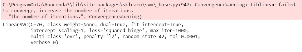
Figure 7.23: Configuration of the linear SVM classifier
- Now, test the performance of the trained model using the test images. This code iterates over each of the test images, then it calculates the LBPH features. Finally, it will pass the extracted features to the model to find the class of the image. In the end, the OpenCV library is used to display the name of the predicted class in a window:
test_data = []
prediction_result = []
for image_path in paths.list_images(test_data_path):
# read the image, convert it to grayscale
image = cv2.imread(image_path)
gray = cv2.cvtColor(image, cv2.COLOR_BGR2GRAY)
# Extract LBPH features
lbp = feature.local_binary_pattern(gray, numPoints,
radius, method="uniform")
(hist, _) = np.histogram(lbp.ravel(),
bins=np.arange(0, numPoints + 3),
range=(0, numPoints + 2))
hist = hist.astype("float")
# normalize histograms
hist /= (hist.sum() + eps)
test_data.append(hist)
prediction = model.predict(hist.reshape(1, -1))
# display the image and the prediction
cv2.putText(image, prediction[0], (10, 30),
cv2.FONT_HERSHEY_SIMPLEX, 0.5, (0, 0, 255))
cv2.imshow("predicted image", image)
cv2.waitKey(5000)
cv2.destroyAllWindows()
The preceding code produces the following output:

Figure 7.24: Prediction results on the test images using the LBPH algorithm
Note
All output will be displayed after 5 seconds in a single window.
In this exercise, we first trained a linear SVM classifier and then used it to predict labels for an unseen dataset/testing dataset. The important thing to remember here is that the classifier was trained based on the features obtained from the LBPH algorithm. This resulted in better performance, even using a model as simple as a linear SVM-based classifier.
Figure 7.25 and Figure 7.26 show a brief overview of the training steps and test steps respectively, used in Exercise 7.05, Object Detection Using the LBPH Method:

Figure 7.25: Training steps in exercise 7.05
As shown in Figure 7.25, the training steps first take color or grayscale images as input. If the input image is a color image, then the next step converts the input image into grayscale; otherwise, the input image is passed to the LBPH feature extraction function. In the next step, the computed features are normalized. Then, the next step instantiates an SVM model. Finally, the model is trained using training images:
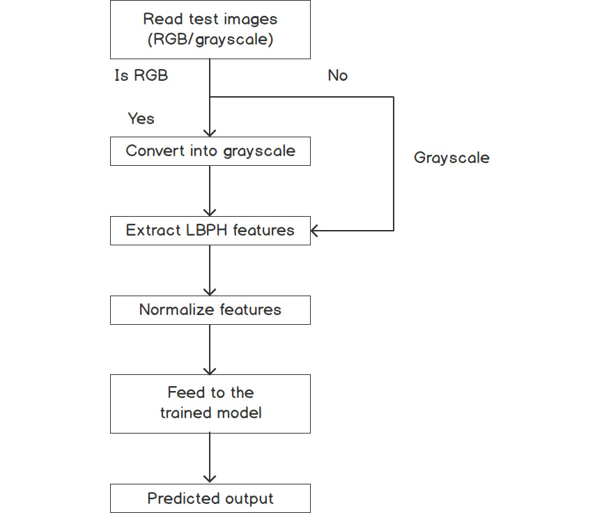
Figure 7.26: Test steps in the exercise 7.05
As shown in Figure 7.26, the test step first takes a new color or grayscale image as input. If the input is a color image, then the next step converts the input image into grayscale; otherwise, the input image is passed to the LBPH feature extraction function. In the next step, the computed features are normalized. Then, the next step feeds the extracted features to the trained model (which is trained during the training steps). Finally, it outputs the category of the input image.
In this exercise, you learned how to implement object detection with LBPH. You built an object detection model for three categories. It is recommended that you add more categories and images to check the performance of the algorithm.
Note
To access the source code for this specific section, please refer to https://packt.live/3dVIOWA.
Next, we will implement a Haar-based object detection model.
Haar Cascades
In Chapter 5, Face Processing in Image and Video, we discussed the Haar Cascades classifier. We implemented face detection using it. Now, we will quickly recap the concepts of Haar Cascades and implement object detection using it. In this algorithm, Haar-like feature extraction is carried out by considering a large set of adjacent rectangular regions of different scales, which then move over an image. At any specific region, pixels in adjacent windows are summed up and the difference of these sums is then used to categorize that region of the image. Generally, areas around the eyes are darker than cheeks. So, one example of Haar features for face detection would be a set of rectangular windows for the eye region and the cheek region. Through this approach, many Haar features are generated. But not all the features are relevant. At this step, a well-known boosting technique – AdaBoost – comes into the picture, which can reduce the number of features to a great extent and can yield only the relevant features out of a huge pool.
Now that we have revised the concepts of Haar Cascades, let's implement car and pedestrian detection models using it.
Exercise 7.06: Object Detection Using Haar-Based Features
In this exercise, we will perform object detection using Haar-based features. In the previous exercise, we used LBPH features to train a support vector classifier that was then used for object detection. In this exercise, we will carry out object detection using pre-trained Haar Cascade classifiers:
Note
Before we go ahead and start working on this, please make sure that you have downloaded the haarcascade_car.xml and haarcascade_fullbody.xml files. These are available at https://packt.live/3j2rYcc.
We will use the cv2.VideoCapture() function to read frames from videos and also from webcams.
- Firstly, open an untitled Jupyter Notebook and name the file Exercise7.06 or object_detection_haar_cascade.
- Start by importing all the required libraries for this activity:
import cv2
- Specify the path of the OpenCV XML files that will be used to detect people and cars in each image. Create a folder named opencv_xml_files and save the haarcascade_car.xml and haarcascade_fullbody.xml files inside that folder:
haarcascade_car = 'opencv_xml_files/haarcascade_car.xml'
haarcascade_fullbody = 'opencv_xml_files/haarcascade_fullbody.xml'
- Next, load the XML file that will be used to detect cars. To detect pedestrians, replace haarcascade_car.xml with haarcascade_fullbody.xml:
car_classifier = cv2.CascadeClassifier(haarcascade_car)
# for pedestrian detection use file
#'opencv_xml_files/haarcascade_fullbody.xml'
# classifier = cv2.CascadeClassifier(haarcascade_fullbody)
- Read frames from the video and detect the cars in it. Currently, a video named cars.avi is being used. Steps 5 - 6 explain how to read frames using video.
Note
cars.avi can be downloaded from https://packt.live/3dPxsDk.
The code is as follows:
cap = cv2.VideoCapture('cars.avi')
# for pedestrian detection
# cap = cv2.VideoCapture('walking.avi')
count = 0
Note that a count variable is used in this code. The purpose of this variable to select every nth frame in a video. Sometimes, we get a video with 30 or more frames per second. It becomes slightly difficult to see the predicted result for each frame, so instead of detecting objects in each frame, we can apply a detection model on every nth frame. Currently, we are detecting every 20th frame, but we can change this to any number.
- In this step, you will read every 20th frame, until the last frame. For each frame, the image will be converted to grayscale. Then, pre-trained files from Step 4 will detect the cars in each frame. Next, a rectangular box will be created around the detected cars with labels on them. Finally, the model will display a stream of frames in a window. The window will be closed once the code reaches the last frames of the input video:
while cap.isOpened():
count +=1
# here 20 means every 20th frame.
if count%20==0:
ret, frame = cap.read()
gray = cv2.cvtColor(frame, cv2.COLOR_BGR2GRAY)
cars=car_classifier.detectMultiScale(gray,1.1, 3)
for (x,y,w,h) in cars:
cv2.rectangle(frame, (x, y), (x+w, y+h), (0, 255, 0), 2)
cv2.putText(frame, 'car', (x, y-10),
cv2.FONT_HERSHEY_SIMPLEX, 0.4, (0, 0, 255))
cv2.imshow('car', frame)
# for pedestrian
#cv2.imshow('person', frame)
# press 'q' to destroy window
if cv2.waitKey(1) & 0xFF == ord('q'):
break
cap.release()
cv2.destroyAllWindows()
Figure 7.27 shows the result of car detection using a Haar Cascades classifier:

Figure 7.27: Detection results on a few frames of the video using the Haar Cascades algorithm
Note
All output will be displayed in a single window.
To access the source code for this specific section, please refer to https://packt.live/2NIOQij.
In this exercise, we used Haar Cascades to detect the cars present in a video frame. This is different from the LBPH method we used in the previous exercise, where we had to train a support vector classifier to detect the objects present in a frame. Here we have used a pre-trained Haar Cascades classifier, and that's why we have effectively only performed the inference step.
Figure 7.28 shows a brief overview of the steps in this exercise:

Figure 7.28: Brief overview of steps in exercise 7.06
The first step creates a video capture object and reads an input file. Then, the second step reads every 20th frame. If the input is a color image, then the next step converts the input image into grayscale; otherwise, it passes each frame into the car detection module. Finally, the last step creates a rectangular box with a label for each car detected in the frame.
In this exercise, you have learned how to implement object (car) detection using the Haar Cascades method in a video. By following the instructions in this exercise, you can also detect humans in a video.
Activity 7.01: Object Detection in a Video Using MobileNet SSD
In this activity, you will implement an object detection model for a recorded video and for some real-time video. You can use any video to detect object instances in each frame. Other than that, a webcam can be used to detect objects in real-time.
The steps to follow to solve the problem have been listed here:
- First, open an untitled notebook and create a file named Activity7.01. We will type out our code in this file.
- Import the necessary Python modules.
- Download the MobileNetSSD_deploy.prototxt file, and the pre-trained MobileNet SSD model: MobileNetSSD_deploy.caffemodel.
Note
The MobileNetSSD_deploy.prototxt and MobileNetSSD_deploy.prototxt files can be downloaded from https://packt.live/2ZvqpdI.
- Load both the downloaded files using OpenCV's dnn module.
- Prepare a dictionary of categories that can be detected by the model.
- Provide the path of the input video to cv2.VideoCapture(path) and read each frame.
Note
The input video, walking.avi, can be downloaded from https://packt.live/3gecS12.
- Perform the pre-processing steps for each frame, such as resizing and converting into a blob, before feeding it to the model.
- Store the model output to a variable (say, detection_result).
- For each frame, the model will return detected instances. Iterate over all the detected instances and check whether the confidence score (probability) of the detected object is greater than the threshold (say, 0.2 or 0.3).
- If the confidence of detection is greater than the threshold, then get the coordinates and category ID of the object from the detection_result variable.
- Note that in the pre-processing step, each image is resized, so to get the locations of the objects in the original frame, scale the coordinates.
- Check whether the category ID is present in the dictionary created in Step 5. If it is, then create a rectangular box around the detected object and label it.
- Display the result in the cv2 window.
- Once these steps are done, replace the path with 0 in cv2.VideoCapture(). It will start using a webcam. Bring your face or any other object in front of the webcam. It will start detecting objects in real-time.
- It is advised to test the results with various input videos.
Once all the steps are completed successfully, you should be able to get the images shown in Figure 7.29 and Figure 7.30. Figure 7.29 shows the prediction results for one of the frames of the input video:

7.29: Sample output of the prediction results for one of the frames of the input video
Figure 7.30 is a sample of how the result would look if you were to use a webcam. For representation purposes, an image of a train was placed in front of the webcam. You are advised to bring any object in front of the webcam from the list that we created in Step 4 of Exercise 7.04, Object Detection Using MobileNet SSD:
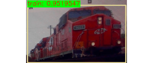
7.30: Sample output of the prediction results using a webcam
Note
The solution for this activity can be found on page 518.
Activity 7.02: Real-Time Facial Recognition Using LBPH
In this activity, you will implement a real-time facial recognition model. The objective is to use a camera to recognize a person in real-time. The solution can be extended to real-world problems. To start with, you can use real-time facial recognition to build an attendance system for offices or schools.
The steps to follow to solve the problem have been listed here:
- First, open an untitled notebook and create a file named Activity7.02.
- Import the necessary Python modules.
- Download the lbpcascade_frontalface.xml file. It will be used for face detection.
Note
The lbpcascade_frontalface.xml file can be downloaded from https://packt.live/3ifLn9j.
- Use the webcam to detect faces and store them in a folder. If you like, you can start by capturing your own face images and storing them in the folder.
- Read the files from the folder and create a set of training images with their respective labels.
- Use the face recognizer module from OpenCV to build a recognizer model.
- Train the model on the training data.
- Again, use the webcam and haarcascade XML files to detect a face and pass this face to the recognizer model and check whether the trained model can recognize the new face correctly.
- Increase the number of unique faces (categories) to check the performance of the model.
Note
As mentioned in step 4, this activity will access your webcam and store the faces of people who are in front of the camera.
Once all the steps are done successfully, you should be able to get the image of a person and their name. Figure 7.31 is a sample representation of how the output should look. So, instead of an emoji, you will see a real face and their assigned name:

Figure 7.31: Example output for this activity
Note
The solution for this activity can be found on page 523.
In this activity, you have learned how to build a real-time facial recognition model. You can extend this solution to build an attendance system in an office or to monitor areas around your home (to check whether unknown people are roaming).
Summary
In this chapter, we discussed the concepts of facial recognition and object detection. In the first part, we discussed three popular classical algorithms for facial recognition. We started with the Eigenface method, and then we discussed its limitations. Then, we moved on to the next method, called Fisherface, and discussed how it solves the limitations of the Eigenface method. We looked into the limitations of Fisherface as well. Finally, we concluded our study of facial recognition with a look at the LBPH method. We have also implemented three different face recognizers using these three methods. We observed that these methods work well if the illumination of images is uniform, and if the face in the image is facing the camera head-on rather than at an angle.
In the second part, we discussed three different object detection algorithms. We started with a recently developed algorithm called MobileNet SSD. In this section, we discussed how SSD performs object detection in a single shot, which makes this algorithm faster than some of its competitors. Then, we discussed how the low complexity of MobileNet makes it a preferred choice for real-time use cases. Moving on, we discussed classical approaches to object detection, such as the LBPH and Haar Cascade methods. We concluded our look at object detection by implementing object detection models using these two classical methods.
In the next chapter, we will discuss Intel's OpenVINO toolkit, a recent addition to the OpenCV module. We will start with an introduction to OpenVINO, where we will discuss the various components of OpenVINO and how to combine it with OpenCV at various steps – image pre-processing, model optimizing, inference engines, and so on. We will also use some pre-trained models present in ModelZoo to build some applications.