
In this section, we will implement a naive strategy based on the number of times a price increases or decreases. This strategy is based on the historical price momentum. Let's have a look at the code:
def naive_momentum_trading(financial_data, nb_conseq_days):
     signals = pd.DataFrame(index=financial_data.index)
     signals['orders'] = 0
     cons_day=0
     prior_price=0
     init=True
     for k in range(len(financial_data['Adj Close'])):
         price=financial_data['Adj Close'][k]
         if init:
             prior_price=price
             init=False
         elif price>prior_price:
             if cons_day<0:
                 cons_day=0
             cons_day+=1
         elif price<prior_price:
             if cons_day>0:
                 cons_day=0
             cons_day-=1
         if cons_day==nb_conseq_days:
             signals['orders'][k]=1
         elif cons_day == -nb_conseq_days:
             signals['orders'][k]=-1

     return signals

 ts=naive_momentum_trading(goog_data, 5)
In this code, the following applies:
- We count the number of times a price is improved.
- If the number is equal to a given threshold, we buy, assuming the price will keep rising.
- We will sell if we assume that the price will keep going down.
We will display the evolution of the trading strategy by using the following code:
fig = plt.figure()
 ax1 = fig.add_subplot(111, ylabel='Google price in $')
 goog_data["Adj Close"].plot(ax=ax1, color='g', lw=.5)

 ax1.plot(ts.loc[ts.orders== 1.0].index,
          goog_data["Adj Close"][ts.orders == 1],
          '^', markersize=7, color='k')

 ax1.plot(ts.loc[ts.orders== -1.0].index,
          goog_data["Adj Close"][ts.orders == -1],
          'v', markersize=7, color='k')

 plt.legend(["Price","Buy","Sell"])
 plt.title("Turtle Trading Strategy")

 plt.show()
This code will return the following output. This curve represents the orders for the naive momentum trading strategy:
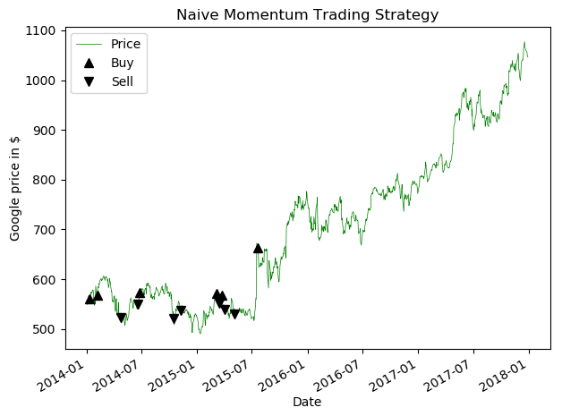
From this plot, the following can be observed:
- The naive trading strategy does not produce many orders.
- We can have a higher return if we have more orders. For that, we will use the following strategy to increase the number of orders.