In total, the nine years of filing history provide us with over 28,000 numerical values. We can select a useful field, such as Earnings per Diluted Share (EPS), that we can combine with market data to calculate the popular Price/Earnings (P/E) valuation ratio.
We do need to take into account, however, that Apple split its stock 7:1 on June 4, 2014, and Adjusted Earnings per Share before the split to make earnings comparable, as illustrated in the following code block:
field = 'EarningsPerShareDiluted'
stock_split = 7
split_date = pd.to_datetime('20140604')

# Filter by tag; keep only values measuring 1 quarter
eps = aapl_nums[(aapl_nums.tag == 'EarningsPerShareDiluted')
                & (aapl_nums.qtrs == 1)].drop('tag', axis=1)

# Keep only most recent data point from each filing
eps = eps.groupby('adsh').apply(lambda x: x.nlargest(n=1, columns=['ddate']))

# Adjust earnings prior to stock split downward
eps.loc[eps.ddate < split_date,'value'] = eps.loc[eps.ddate <
        split_date, 'value'].div(7)
eps = eps[['ddate', 'value']].set_index('ddate').squeeze()
eps = eps.rolling(4, min_periods=4).sum().dropna() # create trailing
                  12-months eps from quarterly data
We can use Quandl to obtain Apple stock price data since 2009:
import pandas_datareader.data as web
symbol = 'AAPL.US'
aapl_stock = web.DataReader(symbol, 'quandl', start=eps.index.min())
aapl_stock = aapl_stock.resample('D').last() # ensure dates align with
                                               eps data
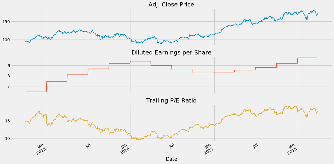
Now we have the data to compute the trailing 12-month P/E ratio for the entire period:
pe = aapl_stock.AdjClose.to_frame('price').join(eps.to_frame('eps'))
pe = pe.fillna(method='ffill').dropna()
pe['P/E Ratio'] = pe.price.div(pe.eps)
axes = pe.plot(subplots=True, figsize=(16,8), legend=False, lw=2);
We get the following plot for the preceding code: