
We have captured the test predictions from the 250 folds and can compute both the overall and a 21-day rolling average:
fig, axes = plt.subplots(nrows=2)
rolling_result = test_result.rolling(21).mean()
rolling_result[['ic', 'pval']].plot(ax=axes[0], title='Information Coefficient')
axes[0].axhline(test_result.ic.mean(), lw=1, ls='--', color='k')
rolling_result[['rmse']].plot(ax=axes[1], title='Root Mean Squared Error')
axes[1].axhline(test_result.rmse.mean(), lw=1, ls='--', color='k')
We obtain the following chart that highlights the negative correlation of IC and RMSE and their respective values:
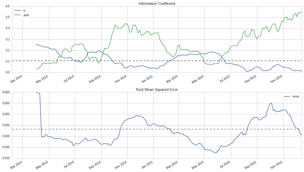
Chart highlighting the negative correlation of IC and RMSE
For the entire period, we see that the Information Coefficient measured by the rank correlation of actual and predicted returns is weakly positive and statistically significant:
