Boosting is an ensemble method, so it creates a set of different classifiers. Imagine that you have m classifiers, we can define a classifier x as:

When we need to evaluate a new observation, we can calculate the average of all m tree's predictions using the following formula:

We can improve this evaluation by adding a weight to each tree, as shown here in this formula:

We can use this mechanism for Regression and also for classification (for example, if the result is higher or equal to one, the observation belongs to class X). For classification, we can also use other mechanisms such as the majority of vote.

Now, we know to ensemble a set of classifiers, but we need to create this set of classifiers. To create different classifiers, we will use different subsets of data.

The most usual boosting algorithm is AdaBoost or adaptive boosting. This algorithm was created by Yoav Freund and Robert Schapire in 1997. In AdaBoost, we start by assigning equal weights to all observations. To create the first tree, we will select a random set of observations. After creating and evaluating the model, we will increase the weight of misclassified observations in order to boost misclassified observations. Now, we can create the second leaner or model by selecting a new random set of observations. After creating each leaner, we will increase the weight of misclassified observations.

To create a boosting model, you have to go to Rattle's Model tab and select the Boost type, as shown in the following screenshot:

Rattle offers different options, the most important ones are:

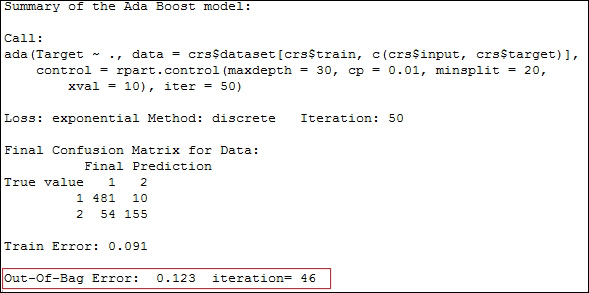
In an ensemble algorithm, Out-Of-Bag Error or OOB Error is a good approach to performance. OOBs are observations that are not in the subset used to create each tree. Rattle uses all observations that aren't in the subset used to create the trees to validate the model. When we see an OOB Error of 0.123, it means that our model correctly classifies 87.7 percent of the observation that wasn't in the random training set.

When we execute the Boost model, Rattle returns information in text form. See highlighted in the following screenshot, the Out-of-Bag Error and iteration values. In our example, the iteration is 46. We ran the example with the variable Number of Trees set to 46; a iteration of 46 and OOB error 0.123 means that with 46 trees, we can achieve a OOB error of 0.123. If we increase the Number of Trees value to 50, we won't be able to achieve a better OOB Error, as shown here:

If you press the button; Errors, Rattle will plot the OOB Error, and you will see how it evolves when you add more trees to the model.

Finally, we've created a set of trees; we can see each tree in the text format or as a plot by pushing the List or Draw button and select the number of trees in the text field, as shown here:

Random Forest is an ensemble method developed by Leo Breiman and Adele Cutler in 2001. This is an ensemble algorithm, so we don't have a single tree, we've a set of trees or a forest. Random Forest combines this set of trees in a single model to improve the performance.

The main idea is to produce a set of trees, introducing some randomness in each tree, and combine all of them to produce a better prediction. The randomness is produced in two different ways; in the set of variables used to split the data in branches, and in the observations used to create (train) the tree.

The basic algorithm, is the same as we've already seen in this chapter, but now we will create a fixed number of trees. We need to decide the Number of Trees value and Rattle will create this many number of trees for us. Before it creates a tree, it randomly selects a set of observations to train the classifier and uses a randomly chosen subset of input variables to split the data. The final result is a set of trees.

In order to predict a new observation, Random Forest evaluates the new observations for each tree. If the target attribute is categorical (classification), Random Forest will choose the most frequent as its prediction. If the target variable is numerical (Regression), the average of all predictions will be chosen.

To create a Random Forest model in Rattle, you have to load a dataset, go to the Model tab, and choose Forest as the model type, as shown here:

After selecting Forest as the model type, press the Execute button to create the model. After executing Random Forest, Rattle creates a summary. The summary contains the following:

We'll see the confusion matrix in the next chapter. Now, we have to see the OOB estimate of the error rate. In the following screenshot, we will see 23 percent as the OOB estimate of error rate. This rate is high, and means our model has low performance, as indicated in this screenshot:

Rattle offers you some options to improve the model. You can choose Number of Trees that the model will create and Number of Variables; in between, Rattle will choose one to split the dataset. We can use the Impute checkbox to control whether observations with missing values are ignored or not.

We've four buttons: Importance, Rules, Errors and OOB ROC. You've seen before that by pressing the Rules button, Rattle converts a tree to a set of rules. In this case, we have a set of trees. For this reason, we've a text field where we can indicate the number of trees. If we write three in the text field and press Rules, Rattle will convert the tree number three, to a set of rules.

The Importance button creates a plot that shows two measures of the variable importance prediction accuracy and Gini index. The Gini index is a measure of the inequality of a distribution. These two measures help us to understand which variables are more useful for predicting a new observation.

There is a trade-off between the error rate and the time needed to create the model. If we choose to create a small number of trees, Rattle will need a small amount of time to create it, but the error rate will be high. If we choose creating a large number of trees, the time needed will be higher, but the error rate will be lower. A good tool to choose the number of trees is the error plot. Press the Error button and Rattle will create an error plot. This plot shows us the evolution of the OOB estimate of error rate when you increase the number of trees. Look at the following screenshot; when the number of trees is small, the error rate is high; by incrementing the number of trees, we will decrease the error rate. In the same plot, we can see the error rate associated with each prediction:

Finally, Sample Size can be used to limit the number of observations necessary to create each tree, or in a classifier, can be used to define the number of observations of each class that will be used. In our credit example, we've 1,000 observations; 700 are classified as 1, and 300 are classified as 2. On average, the number of observations classified as 1 in each sample dataset will be 70 percent. We can use Sample Size to create a different distribution. If you use 200,200 as the Sample Size value, each sample dataset will contain 200 observations classified as 1 and 200 as 2.

Supported Vector Machine (SVM) is a supervised method used for Classification and Regression. SVM looks for the best separation between observations that belong to different classes. The best separation is the one with the higher margin. In the following diagram, you can see a dataset with two classes of observations: stars and circles. On the left-hand side, the observations are divided by a line called Line 1. On the right-hand side, there is the same dataset divided by a line called Line 2:

In this example, our dataset only has two attributes and can be represented in a plane and divided by a simple line, but usually our datasets are more complex and have a lot of attributes. We need to use a hyperplane to divide them.

Usually, different classes in a dataset are not easily separable as on our previous example. For this reason, Kernel Functions are used to preprocess the attributes of the observations to convert into easier separable observations. The performance of the model depends on the Kernel Function used.