
In short-rate modeling, the short rate r(t) is the spot rate at a particular time. It is described as a continuously compounded, annualized interest rate term for an infinitesimally short period of time on the yield curve. The short rate takes on the form of a stochastic variable in interest rate models, where the interest rates may change by small amounts at every point of time. Short rate models attempt to model the evolution of interest rates over time, and hopefully describe the economic conditions at certain periods.
Short-rate models are frequently used in the evaluation of interest rate derivatives. Bonds, credit instruments, mortgages, and loan products are sensitive to interest rate changes. Short-rate models are used as interest rate components in conjunction with pricing implementations, such as numerical methods, to help price such derivatives.
Interest rate modeling is considered a fairly complex topic since interest rates are affected by a multitude of factors, such as economic states, political decisions, government intervention, and laws of demand and supply. A number of interest rate models have been proposed to account for various characteristics of interest rates.
In this section, we will take a look at some of the most commonly used one-factor short rate models used in financial studies, namely, the Vasicek model, Cox-Ingersoll-Ross model, Rendleman and Bartter model, and Brennan and Schwartz model. Using Python, we will perform a one-path simulation to obtain a general overview of the interest rate path process. Other models commonly discussed in finance include the Ho-Lee model, Hull-White model, and Black-Karasinki model.
In the one-factor Vasicek model, the short rate is modeled as a single stochastic factor:
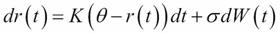
Here, ![]() ,
, ![]() , and
, and ![]() are constants, and
are constants, and ![]() is the instantaneous standard deviation.
is the instantaneous standard deviation. ![]() is the random Wiener process. The Vasicek follows an Ornstein-Uhlenbeck process, where the model reverts around the mean
is the random Wiener process. The Vasicek follows an Ornstein-Uhlenbeck process, where the model reverts around the mean ![]() with
with ![]() , the speed of mean reversion. As a result, the interest rates may become negative, which is an undesirable property in most normal economic conditions.
, the speed of mean reversion. As a result, the interest rates may become negative, which is an undesirable property in most normal economic conditions.
To help understand this model, the following Python code generates a list of interest rates:
""" Simulate interest rate path by the Vasicek model """
import numpy as np

def vasicek(r0, K, theta, sigma, T=1., N=10, seed=777):
    np.random.seed(seed)
    dt = T/float(N)
    rates = [r0]
    for i in range(N):
        dr = K*(theta-rates[-1])*dt + sigma*np.random.normal()
        rates.append(rates[-1] + dr)
    return range(N+1), rates
The
vasicek function returns a list of time periods and interest rates from the Vasicek model. It takes in a number of input parameters: r0 is the initial rate of interest at t=0; K, theta, and sigma are constants; T is the period in terms of number of years; N is the number of intervals for the modeling process; and seed is the initialization value for NumPy's standard normal random number generator.
Assume that the current interest rate is 1.875 percent, K is 0.2, theta is 0.01, and sigma is 0.012. We will use a T value of 10 and N value of 200 to model the interest rates as follows:
>>> x, y = vasicek(0.01875, 0.20, 0.01, 0.012, 10., 200)
>>>
>>> import matplotlib.pyplot as plt
>>> plt.plot(x,y)
>>> plt.show()
After running the above commands, we will get the following output:

In this example, we will run just one simulation to observe what the interest rates from the Vasicek model will look like. As observed, the interest rates did become negative at some point and grew on an average at 0.01.
The Cox-Ingersoll-Ross (CIR) model is a one-factor model that was proposed to address the negative interest rates found in the Vasicek model. The process is given as:
The term ![]() increases the standard deviation as the short rate increases.
increases the standard deviation as the short rate increases.
Now the vasicek function can be rewritten as the CIR model in Python:
""" Simulate interest rate path by the CIR model """
import math
import numpy as np

def cir(r0, K, theta, sigma, T=1.,N=10,seed=777):
    np.random.seed(seed)
    dt = T/float(N)
    rates = [r0]
    for i in range(N):
        dr = K*(theta-rates[-1])*dt +
            sigma*math.sqrt(rates[-1])*np.random.normal()
        rates.append(rates[-1] + dr)
    return range(N+1), rates
Using the same example given in the Vasicek section, assume that the current interest rate is 1.875 percent, K is 0.2, theta is 0.01, and sigma is 0.012. We will use a T value as 10 and N as 200 to model the interest rates as follows:
>>> x, y = cir(0.01875, 0.20, 0.01, 0.012, 10., 200)
>>>
>>> import matplotlib.pyplot as plt
>>> plt.plot(x,y)
>>> plt.show()
Here is the output for the preceding commands:

Observe that the CIR interest model does not have negative interest rate values.
In the Rendleman and Bartter model, the short rate process is given as:

Here, the instantaneous drift is ![]() with an instantaneous standard deviation
with an instantaneous standard deviation ![]() . The Rendleman and Bartter model can be thought of as a geometric Brownian motion, akin to a stock price stochastic process that is log-normally distributed. This model lacks the property of mean reversion. Mean reversion is a phenomenon where the interest rates seem to be pulled back toward a long-term average level.
. The Rendleman and Bartter model can be thought of as a geometric Brownian motion, akin to a stock price stochastic process that is log-normally distributed. This model lacks the property of mean reversion. Mean reversion is a phenomenon where the interest rates seem to be pulled back toward a long-term average level.
The following Python code models the Rendleman and Bartter interest rate process:
""" Simulate interest rate path by the Rendleman-Barter model """
import numpy as np

def rendleman_bartter(r0, theta, sigma, T=1.,N=10,seed=777):
    np.random.seed(seed)
    dt = T/float(N)
    rates = [r0]
    for i in range(N):
        dr = theta*rates[-1]*dt +
             sigma*rates[-1]*np.random.normal()
        rates.append(rates[-1] + dr)
    return range(N+1), rates
We will continue to use the example from the previous sections and compare the model. Assume that the current interest rate is 1.875 percent, theta is 0.01, and sigma is 0.012. We will use a T value as 10 and N as 200 to model the interest rates as follows:
>>> x, y = rendleman_bartter(0.01875, 0.01, 0.012, 10., 200)
>>>
>>> import matplotlib.pyplot as plt
>>> plt.plot(x,y)
>>> plt.show()
The following graph is the output for the preceding commands:

In general, this model lacks the property of mean reversion and grows toward a long-term average level.
The Brennan and Schwartz model is a two-factor model where the short-rate reverts toward a long rate as the mean, which also follows a stochastic process. The short-rate process is given as:
It can be seen that the Brennan and Schwartz model is another form of a geometric Brownian motion.
Our Python code can now be implemented as follows:
""" Simulate interest rate path by the Brennan Schwartz model """
import numpy as np

def brennan_schwartz(r0, K, theta, sigma, T=1., N=10, seed=777):
    np.random.seed(seed)
    dt = T/float(N)
    rates = [r0]
    for i in range(N):
        dr = K*(theta-rates[-1])*dt +
            sigma*rates[-1]*np.random.normal()
        rates.append(rates[-1] + dr)
    return range(N+1), rates
Assume that the current interest rate is 1.875 percent, K is 0.2, theta is 0.01, and sigma is 0.012. We will use a T value as 10 and N as 10000 to model the interest rates as follows:
>>> x, y = brennan_schwartz(0.01875, 0.20, 0.01, 0.012, 10.,
...                         10000)
>>>
>>> import matplotlib.pyplot as plt
>>> plt.plot(x,y)
>>> plt.show()
After running the above commands, we will get the following output:
