
In the options pricing methods we learned so far, a number of parameters are assumed to be constant: interest rates, strike prices, dividends, and volatility. Here, the parameter of interest is volatility. In quantitative research, the volatility ratio is used to forecast price trends.
To derive implied volatilities, we need to refer to Chapter 3, Nonlinearity in Finance where we discussed root-finding methods of nonlinear functions. We will use the bisection method of numerical procedures in our next example to create an implied volatility curve.
Let's consider the option data of the stock Apple (AAPL) gathered at the end of day on October 3, 2014, given in the following table. The option expires on December 20, 2014. The prices listed are the mid-points of the bid and ask prices:
|
Strike price |
Call price |
Put price |
|---|---|---|
|
75 |
30 |
0.16 |
|
80 |
24.55 |
0.32 |
|
85 |
20.1 |
0.6 |
|
90 |
15.37 |
1.22 |
|
92.5 |
10.7 |
1.77 |
|
95 |
8.9 |
2.54 |
|
97.5 |
6.95 |
3.55 |
|
100 |
5.4 |
4.8 |
|
105 |
4.1 |
7.75 |
|
110 |
2.18 |
11.8 |
|
115 |
1.05 |
15.96 |
|
120 |
0.5 |
20.75 |
|
125 |
0.26 |
25.81 |
The last traded price of AAPL was 99.62 with an interest rate of 2.48 percent and a dividend yield of 1.82 percent. The American options expire in 78 days.
Using this information, let's create a new class named ImpliedVolatilityModel that accepts the stock option's parameters in the __init__ constructor method. Import the BinomialLROption class that we created for the Leisen-Reimer binomial tree covered in the earlier section of this chapter. Also, import the bisection.py file that we created using the bisection function covered in Chapter 3, Nonlinearity in Finance.
The _option_valuation_ method accepts the strike price K and the volatility value sigma to compute the value of the option. In this example, we are using the BinomialLROption pricing method.
The get_implied_volatilities public method accepts a list of strike and option prices to compute the implied volatilities by the bisection method for every price available. Therefore, the length of the two lists must be the same.
The Python code for the ImpliedVolatilityModel is given as follows:
"""
Get implied volatilities from a Leisen-Reimer binomial
tree using the bisection method as the numerical procedure.
"""
from bisection import bisection
from BinomialLROption import BinomialLROption

class ImpliedVolatilityModel(object):

    def __init__(self, S0, r, T, div, N,
                 is_call=False):
        self.S0 = S0
        self.r = r
        self.T = T
        self.div = div
        self.N = N
        self.is_call = is_call

    def _option_valuation_(self, K, sigma):
        # Use the binomial Leisen-Reimer tree
        lr_option = BinomialLROption(
            self.S0, K, self.r,  self.T, self.N,
            {"sigma": sigma,
             "is_call": self.is_call,
             "div": self.div})
        return lr_option.price()

    def get_implied_volatilities(self, Ks, opt_prices):
        impvols = []
        for i in range(len(Ks)):
            # Bind f(sigma) for use by the bisection method
            f = lambda sigma:
                self._option_valuation_(
                    Ks[i], sigma) - opt_prices[i]
            impv = bisection(f, 0.01, 0.99, 0.0001, 100)[0]
            impvols.append(impv)
        return impvols
if __name__ == "__main__":
Using this model, let's find out the implied volatilities of the American put options using this particular set of data:
>>> # The data
>>> strikes = [ 75, 80, 85, 90, 92.5, 95, 97.5,
...             100, 105, 110, 115, 120, 125]
>>> put_prices = [0.16, 0.32, 0.6, 1.22, 1.77, 2.54, 3.55,
...               4.8, 7.75, 11.8, 15.96, 20.75, 25.81]
>>>
>>> model = ImpliedVolatilityModel(99.62, 0.0248, 78/365.,
...                           0.0182, 77, is_call=False)
>>> impvols_put = model.get_implied_volatilities(strikes,
                                             put_prices)
The implied volatility values are now stored in the impvols_put variable as a list object. Let's plot these values against the strike prices so that we can get an implied volatility curve:
>>> import matplotlib.pyplot as plt
>>> plt.plot(strikes, impvols_put)
>>> plt.xlabel('Strike Prices')
>>> plt.ylabel('Implied Volatilities')
>>> plt.title('AAPL Put Implied Volatilities expiring in 78 days')
>>> plt.show()
This would give us the volatility smile, as shown in the following figure. Here, we have modeled a Leisen-Reimer tree with 77 steps, each step representing one day:
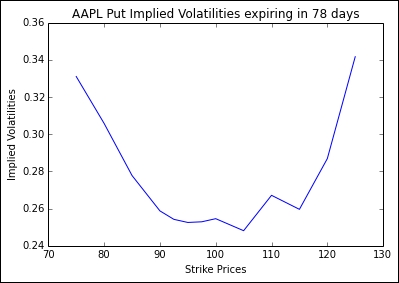
Of course, pricing an option daily may not be ideal since markets change by fractions of a millisecond. We used the bisection method to solve the implied volatility as implied by the binomial tree, as opposed to the realized volatility values directly observed from market prices.
Should we fit this curve against a polynomial curve to identify potential arbitrage opportunities? Or extrapolate the curve to derive further insights on potential opportunities from implied volatilities of far out-of-the-money and in-the-money options? Well, these questions are for options traders like you to find out!