Chapter 10

Valuation of the Target Company Using the Black–Scholes Model

In the framework of a merger and acquisition (M&A), a real call option gives the acquiring company the right, not the obligation, to acquire the target during the time the call option is valid.

As discussed in Chapter 9, one could use a real call option in valuing a target company. Here we discuss the Black–Scholes model for option pricing by first using an example of an option involving stocks and then by another example that illustrates valuation of a potential target firm.

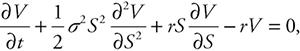
Black and Scholes (1973) developed a model for pricing the fair value of European options. The model is a partial differential equation, which describes the dynamics of option price adjustment within the time to expiration of the option. The derivation of Black–Scholes option pricing formulas is beyond the scope of the study. It suffices to say that the Black–Scholes stochastic differential equation has the following form:

(10.1)

where V is the investor’s long position in one option, s is the standard deviation or a measure of volatility of the underlying asset of the option, S is the asset price, t is time, and r is the risk-free interest rate (interest rate on U.S. Treasury bills).

Pricing the option requires that the aforementioned differential equation be solved. However, an analytical closed form solution1 for some of the stochastic differential equations modeling the dynamics of the option may not exist. For example, American and Asian options2 do not have analytical, closed form solutions (Richardson 2009). In such cases, one must use one of the numerical methods in solving the differential equations. These numerical methods include finite difference, binomial,3 and Monte Carlo methods. However, discussions of these techniques are beyond the scope of the present work.

The analytical solutions to the Black–Scholes formulas for European call (c) and put (p) options for nondividend paying stocks are4

(10.2)

(10.3)

where

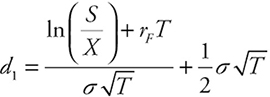(10.4)

(10.5)

The terms in the formula are defined below:

c = European call option price

p = European put option price

S = present value of incremental cash flows (current stock price in call option)

X = investment to create the option (exercise price)

s = volatility of cash inflows (standard deviation of stock price)

T = life of the option

rF = risk-free interest rate

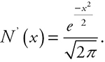
N(x) = the cumulative probability distribution function for a standard normal distribution. See Figure 10.1.

A number of points concerning the option formulas should be kept in mind. We list these important notes.

•The standardized normal probability distribution has a mean 0 and a standard deviation of 1.

•N(x) indicates the probability of a random variable assuming a value less than x or its standardised value Z.

•In the preceding graph, the probability of a random variable x ≤ 1 (or its standardized value Z≤1) is the area under the curve to the left of the vertical line, where Z=1.

•The table for N(x) appears in statistical textbooks, or can be calculated by the NORMSDIST function in Excel.

•The value of N(d) falls in the unit interval: 0 ≤ N(d) ≤ 1 with N(−∝) = 0, 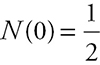, and N(+∝) = 1.

•Note that because of the symmetric nature of the normal probability distribution, (1 – N(d)) = N(–d).

•The term N(d1) is the probability of the future value of the underlying asset that is conditional on where ST is the asset price at the expiration date. N(d2) measures the probability that the option will be exercised, which also implies that call option is in-the-money; otherwise, when the call option would not be exercised.

Calculation of Normal Distribution Using Approximation Method

When one does not have access to a table of area under the curve of a normal distribution or Excel spreadsheet software is not available, one could calculate the cumulative normal distribution function by polynomial approximation to sixth decimal accuracy using the following formula:

(10.6)

and

(10.7)

where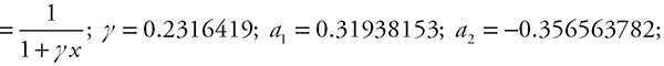

and

(10.8)

Note that the values of the constants g and ai i = 1,2,…,5, are given. See Abramowitz and Stegan (1972).

Example 10.1

Let Z = 1. Calculate the area under the normal distribution function for this random variable using the polynomial approximation method.

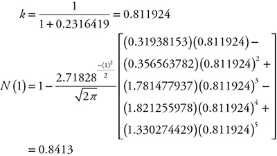
Does the number in the table of areas under the normal curve for Z = 1 confirm this value? The answer is yes. The area under the curve or Z from −∞ to 0 equals 0.5 and from 0 to 1 equals 0.34136. Combining the area of the curve from 1 to −∞ gives the value of 0.8413.

Example 10.2

The stock price 6 months from the expiration of an option is $42, the exercise price of the option is $40, the risk-free interest rate is 0.1 per annum, and the volatility is 0.2 per year. Calculate the call option price for this stock.

Solution

The data in the problem are given below:

Next using values for d1 and d2, and formula for the call option, we have: C = 42N(0.7693) – 38.049N(0.6278).

Note 1:

Note 2: Using a table for standard normal distribution, we get

N(0.7693) = 0.7791,

N(0.6278) = 0.7349,

C = (42)(0.7991) – (38.049)(0.7349) = 4.76.

The stock price must increase $2.76 above its current price of $42, for the purchaser of the call to break even.

Estimating Volatility of the Returns on the Underlying Asset from Historical Data

Another important variable in the Black–Scholes formula to consider is the variance of the rate of return on the underlying asset of the options. This is a measure of volatility of the returns on the underlying asset of the option and measures our uncertainty about the returns on the investment.

To estimate the variance of the rate of the return on the underlying asset, let us suppose that we have n observations in our data set. Let Si represent the stock price at the end of the ith interval, where i = 1,2,…,n. Then let the returns to the stock be ui such that

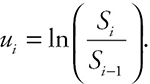(10.9)

Let s represent the estimated standard deviation of ui, so that

(10.10)

where is the mean of ui. Note that ui = ln Si − ln St−1 approximately measures the rate of change (returns) of the stock price.

Time Variability of Volatility of Financial Time Series

The estimated values of and s in Formula 10.10 are dependent on the time series observations of the stock price. This means that the expected value and variance of the time series are not constant but are time-varying. For example, if we calculate the mean and variance of stock price of Citigroup, for example, for two periods, say daily closing prices for 2012 and for 2013, we will obtain two different volatility measures. Hence, the mean and variance of the stock price time series change over time and show periods of high and low volatility. Moreover, investors are interested in volatility of financial assets for the period they wish to hold the assets, and not for a historical period. Accordingly, note that in the following discussions the volatility of stock prices is time dependent.

Based on assumptions about the returns of the underlying assets of options, Black and Scholes derived the probability distribution of the returns on the underlying assets. First, the Black–Scholes model assumes that asset prices in general (financial asset prices in particular) follow random walk processes. Second, the model assumes that the returns on the underlying asset in a short period signified ∆t are normally distributed, and third, it is assumed that the returns on the asset in two nonoverlapping periods are independent. Specifically, this in the discrete time framework, implies that

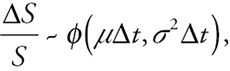(10.11)

where ∆S is the change in the price of the underlying asset S during a very short time ∆t, s2 is the variance of the asset price, and μ is the expected return on the asset during time ∆t. This implies that the variance of the returns is proportional to ∆t.

Note that the fraction on the left side of the expression is the percentage rate of change in the asset price, the term on the right side of the expression represents a normal distribution with μ∆t being the mean of the returns, and s2∆t representing the variance of the stock price series. Expressing it differently, relationship 10.11 states that the rate of return on an asset is proportional to the mean and variance of the distribution of the asset price observations during the relevant time.

The assumptions leading to the expression 10.11 describing the distribution of asset returns imply that the stock price will have a lognormal distribution at any future period. A lognormal distribution is skewed to the right, where the random variable S ≥ 0. By logarithmic transformation, we exclude the cases where the stock price could assume a negative value under normal probability distribution. After all, the worst-case scenario for investment in an asset is that its price falls to 0 and the asset becomes worthless.

A random variable with the distribution property, which cannot assume a negative value, has a natural logarithm that is normally distributed. The assumptions of the Black–Scholes model for the asset prices (previously stated) imply that lnS_T is normal, where ST is the asset price during any length of time T = t − t∗, t is the current time, and t∗ is the end of the investment (the time of selling the investment asset) in future.5 The derivation of the formulas for the mean and standard deviation of ln ST is beyond the scope of this book, and they are shown to be

respectively, where S0 is the current stock

price (Hull 2011). Moreover, the probability distribution of ln ST is written as

(10.12)

Accordingly, we could write the standard deviation of ui based on the historical data, in time t approximately as , where t is the length of time interval in years. Hence we can write

(10.13)

where is an estimate of s, and t is the length of time in years.

Note that the value of the standard deviation depends on time t. As t increases, the standard deviation of the random variable ui declines.

Example 10.3

Consider a stock with an annual expected return of 25 percent and a volatility (standard deviation) of 30 percent per year. Calculate the ­following:

a. The probability distribution of the average rate of return on stock for 6 months

b. The probability distribution of the average rate of return on stock for 4 years

Solution

a.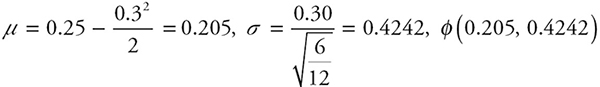

b.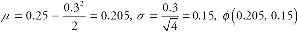

As can be seen from the estimated values, the expected rate of return remains constant, but the volatility tends to decrease, the longer the asset is held.

Example 10.4

a. Specify the probability distribution (calculate the mean and standard deviation) of a stock with an initial price of $50, an expected annual return of 20 percent, and a volatility of 15 percent per annum, for a 6-month duration.

b. Construct a 95 percent confidence interval for the stock price for 6 months.

In solving this problem, we first use Formula 10.12. Note that in this

example , that is, 6 months.

The knowledge of distribution of a random variable is very useful in practice. For instant, an investor may wish to assess the range of values the price of a stock may vary by determining the maximum and minimum limit of its variation. To achieve this goal, one should construct a confidence interval for the stock price.

To construct a 95 percent confidence interval, we use the central limit theorem, a statistical theorem, which states that 95 percent of the sample means from a population, regardless of the shape of its distribution, falls within 1.96 standard deviations of its mean. This implies that Since the estimated mean and standard deviation of the prices for the stock in the problem are based on one sample of observations of the population (population in the context of the time series of a stock’s price refers to prices for the stock for all times), we use the central limit theorem to construct a confidence interval for the stock price:

Of course, this confidence interval defines the range in which the natural log of the stock price will fall. We need to calculate the interval for the actual stock price.

Taking the antinatural logarithm of the expression we have

Accordingly, one can be 95 percent confident that the stock price will fall somewhere in the interval between $44.6358 and $67.6303 within the next 6 months.

The Use of Trading Days and Calendar Days in Volatility Estimation

Studies have shown that volatility of stock prices is much higher stock exchanges are open for trading compared to the time they are closed.6 This has led to the practice of considering only the trading days rather than the calendar days in the calculation of volatility of asset prices using historical data. Accordingly, the formula for calculation of annual volatility V a is given below:

(10.14)

where V td is the volatility per trading day and 252 is the number of trading days per year for stocks.

Note that the life of an option is measured in trading days as well as in calendar days. Moreover, T for the options is measured as follows:

T = (number of trading days until option maturity)/252.(10.15)

To illustrate how to estimate volatility of the price of an underlying asset for options using historical data, we use an example.

Example 10.5

The closing data for Citigroup daily stock price for 21 consecutive trading days appear in the table below.

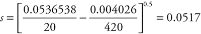
a. Estimate the standard deviation of the daily return.

b. Estimate the annual volatility of the stock price.

c. Estimate the daily volatility of the stock price.

a. The standard deviation of the daily return is

b. Assuming the existence of 252 trading days per year, the annual volatility of the stock is calculated as follows: or slightly greater than 82 percent.

c. The volatility of the stock return in one day is

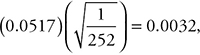or the stock return has 0.32 percent

daily volatility.

How is the standard deviation used in practice? To illustrate the use of the volatility measure, let the stock price be equal to $31.60. Then a one standard deviation move in the stock price in one day is 31.6×0.0032 = $0.00512. As an example, we can cite application of standard deviation as a measure of risk in value at risk analysis.

How Is the Option Value Used in M&A Decision Making?

After valuing the call or put options, the net present value (NPV) is calculated using the following formula:

Total NPV = present value − investment + option value.

Example 10.6

A company plans to invest in a project, and seeks to analyze the returns if it postpones investment for 2 years. The data for the investment projects appear below. Using the NPV and real option methods, calculate the investment outcomes.

Investment in year 2 = $50 million

Present value of incremental cash flows = $40 million

Cost of capital = 10 percent

Risk-free rate = rF = 3.7 percent

Time to maturity = T = 2 years

Strike price = X = $50

Standard deviation = s = 0.15

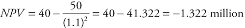
The NPV Method

Real Option Method

Using Formulas 10.4 and 10.5, we calculate d1 and d2 as well as the area under the standard normal distribution function:

Then we use Formula 10.2, the formula for the European call option:

Accordingly, the NPV of the investment adjusted for the option value is –0.022 million, while the NPV of the investment is a negative return of $1.322 million.

Estimating risks associated with an acquisition emerging from the volatility of cash flows is a challenging task in practice. However, the variance used in the Black–Scholes model can be estimated in several ways. One way is to calculate the variance of the stock prices of the firms in the target firm’s industry. For example, an automobile company may use the average of variance of the stock prices of similar automobile companies. Another approach is estimation of the variance of cash flows of similar prior investments. For example, a petroleum exploration company may consider the variance of the cash flows of prior oil exploration projects. A third way is estimation of a measure of volatility of cash flow by the Monte Carlo simulation method.

In a Monte Calro simulation, many alternative scenarios for the net cash flows are estimated by simulating sales, costs, discount factor, or cost of capital, among other factors. The discussion of Monte Carlo is beyond the scope of this book.

Examples of real option valuation in M&As

In this section, we will use examples depicting scenarios for illustration of how one would use real call and put options in target valuation with the option to expand, to delay, and to abandon.

Valuing an Option to Expand

Mardaka Company is negotiating with Zanaca Company, a biotechnology firm, to acquire Zanaca. Based on NPV calculation of Zanaca cash flows, Mardaka can justify the maximum payment of $100 million for Zanaca. However, Zanaca demands a price of $120 million for concluding a deal. Further due diligence by Mardaka shows that combining the resource and technologies of the two companies would lead to more accelerated growth in Zanaca’s cash flows. Retooling Zanaca’s manufacturing operations, with an estimated cost of $100 million, the acquiring company anticipates a high rate of growth in sales. The present value of Zanaca’s cash flows from retooling is estimated to be $80 million. Given the situation, Mardaka cannot justify paying $120 million to conclude the deal.

Subsequent analysis shows, however, that if Zanaca employs ­Mardaka’s new technology, it would acquire the dominant market share changing the market reality altogether. Mardaka believes that it is unlikely that the competitors would develop Zanaca’s technology for another 10 years, a period that allows Mardaka to take full advantage of Zanaka’s ­technology for generating higher sales revenues. It is known that the variance of cash flows for the other firms in the industry is 25 percent. The current government bond yield to maturity is 5 percent. Zanaca’s patent on the technology will expire in 10 years, which in essence, gives an option with a 10-year expiration date to Mardaka.

Calculate the value of call option to Mardaka, the option to expand by retooling Zanaca’s operations. Should it pay the asking price of $120 million?

Solution

The data of the problem are as follows:

Value of the asset (present value of cash flows from retooling Zanaca’s operations) S = $80 million

Exercise price (present value of the cost of retooling Zanaca’s operations or investment to create the option) X = $100 million

Variance of cash flows s2 = 0.25

Time to expiration T = 10 years

Risk-free interest rate rRF = 0.05

Using the Black–Scholes formula for call option, we have

,

where

The NPV of investment in retooling Zanaca’s manufacturing operations plus the value of the call option is calculated as 80 – 100 + 50.08 = $30.08. Therefore Mardaka is justified to pay up to 120 + 30.08 = $150.08 million to acquire Zanaca.

Note: In calculating N(d1) and N(d2), implement the following steps.

1.Consider di, i = 1,2, as the Z-value and look up a table of areas under the normal distribution curve. In the previous example, for Z = 0.9655, N(0.9655) = 0.3315, and for Z = −0.6156, N(-0.6156) = 0.2291

2.Find the area under the curve for the Z-value.

The area under the curve to the left of Z = 0.9655 is (0.5 + 0.3315) = 0.8315.

The area under the curve to the left of Z = −0.6156 is equal 0.2709, that is (1.0–0.5–0.2291) = 0.2709.

Valuation of Real Call Option to Delay

In the real option to delay investment, the underlying asset is the exclusive right to acquire the target firm. The current value of the asset is the present value of the cash flows from undertaking the project now (S). The option’s exercise price is the initial investment in the project (X). The acquiring firm exercises the call option to delay when it decides to postpone investment in the project. The option to delay expires at the time exclusive right to delay expires. However, the delay in investing has an opportunity cost of not having the cash flows during the delay. The annual opportunity cost of delaying the project is 1/T, for an option that expires in T years.

The presence of the opportunity cost of delaying the investment requires that the formula for the European call option be adjusted. This adjustment of the formula is similar to the effect of dividend payment of stocks on the call price. It is well-known that on the day payment and size of dividend are announced, the stock price drops by the amount of dividend. As a result, the value of the call option on the stock that is to receive dividend is reduced, while the value of the put option on the same stocks is increased. Accordingly the call option formula with the opportunity cost of delaying the investment changes to

(10.16)

where D is the dividend yield or opportunity cost. Note that corresponding to the change in the formula for the call option to delay, the formulas for d1 and d2 change as follows:

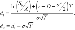(10.17)

Example 10.7

Being an active player in the M&A market, Mardaka Company considers the acquisition of Laukoy Company, a pharmaceutical enterprise, which has developed a new Alzheimer-fighting drug. The drug has been approved by the government food and drug regulatory agency. The marketing research indicates that this new drug will face a low demand initially due to the existing drugs for the disease. However, it is anticipated that the demand for the new drug will have exponential growth in several years when new applications are identified. Identification of new applications, however, requires $100 million initial investment in research and development. Mardaka Company can delay the investment until the management of the company becomes more confident in the actual growth for the demand for the drug. Moreover, it is believed that it may take 10 years before the competing firms produce a new drug for the same applications.

It is estimated that if the new growth for the drug does not materialize, the NPV of Laukoy Company will be $80 million. In such a case, Mardaka’s acquisition of Laukoy is not sensible. The cash flows from previous drug introduction have a variance of 50 percent of the present value of the cash flows. Simulating alternative growth paths for the cash flows generated from the sales of the new drug shows an expected value of $90 million. The 10-year risk-free interest rate is 10 percent.

In spite of the negative NPV of $10 million associated with acquisition of the target, does the value of the call option to delay the initial investment of $100 million warrant acquisition of Laukoy Company?

Solution

Asset value (present value of the expected cash flows from the new drug) S = $90 million

Exercise price (investment required to fully develop the new drug:

strike price) X = $100 million

Variance of cash flows s2 = 0.50

Time to expiration T = 10 years

Risk-free interest rate rRF = 0.10

Opportunity cost of delaying project

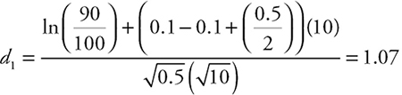
First, calculate the area under the normal curve for d1 = 1.07 and d₂ = –1.165

N(1.07) = 0.5 + 0.2794 = 0.7794

N(–1.165) = 0.5 – 0.377 = 0.123

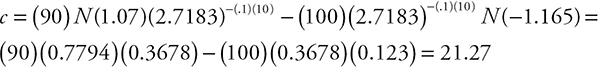
The value of the call option to delay is $21.27 million. Hence the NPV of the acquisition is (S – X + c) = (90 – 100 + 21.27) = 11.27 million. Therefore, Mardaka should acquire Laukoy Company.

Real Option to Abandon

Situations where the acquiring enterprise has the option to abandon the target are tantamount to having real put options, which is the right to sell. Under such circumstances, the decision rule to continue or abandon consists of comparing the value of continuing the project to its liquidation or sale value. The project should continue if its value is greater than the revenue generated by its sale; otherwise, the project should be abandoned.

The real options involving the right to abandon require that the opportunity cost of investment for the period starting from the time of investment until the time of abandonment be included in valuation of the option. As a result, the Black–Scholes formula for a put option is modified as follows:

where now the d1 formula has changed to

To illustrate how the put options in M&As work, let us use an example.

Example

Exploratory work by the National Petroleum Exploration Company (NPEC) has identified a large petroleum reserve in an oil producing country. To fully develop the resource, NPEC requires $500 million dollars, which is beyond the available financial resource of the company. Global Resources International (GRI) is interested in investing in NPEC; however, the preliminary estimate of cash flow from the extraction of petroleum indicates an NPV of only $500 million (S = $500 million). To attract GRI to invest in the extraction project, the NPEC has offered a $250 million real put option (X = $250 million) to GRI, giving the latter the right to sell its shares to NPEC any time on or before the expiration date of the put option, which is 5 years7 T = 5). The put option limits the downside risk to NPEC. The variance of the present value of future cash flows is estimated to be 20 percent (s2 = 0.2). Since the value of the reserve will diminish over time because of the extraction of petroleum, the present value of the investment will diminish as fewer numbers of cash flows remain with the passage of time. Therefore, one should include the opportunity cost of the right to abandon the project. We assume the opportunity cost as 1/n, where n is the number of remaining years of profitable reserves. Let the risk-free interest rate be 5 percent. Is the value of the put option high enough to justify investment in the petroleum extraction project?

Solution

Present value of GRI’s investment in NPEC S = $500 million

Exercise price of put option X = $250 million

Time to expiration of put option T = 5 years

Variance s2 = 0.2

Opportunity cost

Risk-free interest rate r= 0.05.

Using the modified formula for the put option, we have

.

The NPV (S – X + p) = (500 – 250 + 76.20) = 326.20 million justifies the investment. Note that the value of the put option is the additional value created by reducing the risk of the undertaking.

Valuation Challenges

The preceding discussions about the methods of valuation of target enterprises are analytical and as such abstract from the complexity of reality. However, valuation of firms involves a number of practical complications, which the members of the acquisition team should recognize. We discuss these valuation challenges, which appear in all countries, particularly in the emerging economies.

These challenges include:

•Assessing regulatory and market risks

Assessing regulatory and market risk is a challenging task because prediction of the changing macroeconomic and policy environments is difficult and in many situations impossible. For example, we refer the reader to the regulatory obstacles CITIC, a Chinese company, faced in Australia after the initial capital investment, which is discussed in Chapter 5.

•Unreliable historical financial data

In many cases, the required data for valuation analysis may not be available. However, in cases when data do exist, their reliability might be questionable, especially in M&As in the emerging economies.

•Collection of debts

The uncertainty associated with collection of debt could pose additional problems. This is particularly true in many emerging economies, where the contract laws are not well-developed or the legal system is not inclined to enforce the contract laws in a timely manner.

•Questionable capitalization of expenses

In some instances, the target company might have considered day-to-day expenses, such as expenses related to copying machines, as capital investment. Such false capitalization would distort value of the target and must be identified.

•Inadequate accounting of inventories and receivables

Inventories and accounts receivable constitute a major part of a company’s asset. Therefore detail accounting of these items is important for accurate valuation of the target firm. Moreover, the accounting methods for valuation of inventories are not universal and vary based on the accounting systems used by different countries.

The accounts receivable should be analyzed in determining the creditworthiness of the target company’s customers.

•Hidden costs, particularly the cost of labor fringe benefits

Hidden costs such as fringe benefits for the employees could distort valuation of the target firm. Accordingly, detailed due diligence of hidden costs must be performed before conclusion of an agreement.

•Unreasonable assumptions about financial projections

Cash flows are the cornerstone of the valuation of an enterprise. Unreasonable assumptions in projection of future cash flows would result in overvaluation of the target company.

•Inadequate financial modeling training of financial model developers

Financial modeling requires skilled analysts. Analysts with inadequate training and knowledge about financial modeling may provide erroneous financial models and results.

•Unproductive investments in assets such as investment in noncore businesses

Inadequate attention in determining whether every asset of the target is essential for the core business would result in overvaluation of the target firm. The acquiring company should structure a deal so that only the relevant assets of the target for its core business are acquired.

•Significant contingent liabilities such as tax-related issues and guarantees to third parties

A contingent liability refers to a liability that may arise upon occurrence of a certain event. For example, a company faces a contingent liability if the product it markets may cause harm to the consumers of the product. The acquiring company should require the target to disclose any potential liability, pending lawsuits, exposure to potential claims, breach of contracts it may have committed, and all claims and liabilities that may not have been disclosed in the financial statements of the target company.

•Valuation of intangible assets

Intangible assets are important determinants of the profitability of a company and should be considered in valuation of the target firm. Intangible assets appear in a variety of forms including marketing-related (trademarks, brand names, service marks, logos, and agreements with the competitors not to compete); customer-related (customer contracts and relationships, customer lists, databases, open purchase orders, distributors, and sales routes); contract-based: (franchise and licensing agreements, permits and contracts, and supplier contracts); technology-based (process and product innovation patents, and related technical documentation, patent applications, proprietary processes and technology, computer software, and copyrights); and artistic-related (musical composition, literary composition, and film copyrights).

Valuation of intangible assets is a demanding task and should be done by professionals who specialize in this field. We refer the interested reader to ACCUVAL Corporate Valuation and Advisory Services (2013).

•Financial derivatives and instruments

Increasing use of financial instruments, such as financial derivatives, by companies for management of assets and liabilities in recent years requires critical examination of these instruments by the acquisition team.

Summary

This chapter dealt with a number of important topics including valuation of financial call and put options using Black–Scholes formulas, estimating volatility of returns on the underlying asset from historical data, and use of real options in valuation of target under alternative scenarios of options to expand, to delay, and to abandon. Moreover, challenges in company valuation in cross-border M&As were discussed. Finally, using examples, the differences in company valuation with and without real options were illustrated.